1.3 Probability of an Event

Key Terms

Probability（機率）

A number from 0 to 1 that describes how likely an event is to occur.

Event probability（事件機率）

The probability that a particular event occurs. We write it as \(P(A)\).

Equally likely outcomes（等可能結果）

Outcomes that have the same chance of occurring.

Favorable outcomes（有利結果）

Outcomes that belong to the event we are studying.

Total outcomes（全部可能結果）

All possible outcomes in the sample space.

Relative frequency（相對次數）

The fraction of trials in which an event actually occurs.

Certain event（必然事件）

An event that must occur.

Impossible event（不可能事件）

An event that cannot occur.

Loaded die（不公平骰子）

A die whose faces do not all have the same probability.

1.3.2 Learning Outcomes

After completing this section, students should be able to:

• explain probability in simple words;

• explain what \(P(A)\) means;

• identify the possible range of a probability;

• identify certain and impossible events;

• calculate probability when outcomes are equally likely;

• distinguish favorable outcomes from total outcomes;

• explain when the formula \(P(A)=n/N\) can be used;

• calculate and interpret relative frequency;

• explain why relative frequency may differ from theoretical probability;

• calculate an event probability when outcomes are not equally likely.

1.3.3 From Sample Space to Probability

In the previous sections, we studied the sample space and events.

A sample space tells us what can happen.

An event tells us which outcomes we are interested in.

Now we study how likely that event is to happen.

The main relationship is:

Sample Space -> Event -> Probability

Suppose \(A\) is an event.

We write

\[P(A)\]

to mean:

the probability that event \(A\) occurs.

For example, if \(A\) means roll an even number, then \(P(A)\) means the probability of rolling an even number.

1.3.4 Probability and Its Basic Properties

Probability is a number that describes how likely an event is.

Every probability is between 0 and 1.

Note

Probability of an event

\[0 \leq P(A) \leq 1.\]

The two endpoints have special meanings.

If an event is impossible,

\[P(\varnothing)=0.\]

If an event is certain,

\[P(S)=1.\]

Therefore:

• a probability near 0 means the event is unlikely;

• a probability near 1 means the event is likely;

• a probability of 0 means the event cannot occur;

• a probability of 1 means the event must occur.

A probability between 0 and 1 means that the event is possible, but it is not certain.

1.3.5 Example 1: Roll One Fair Die

Suppose we roll one fair six-sided die.

The sample space is

\[S=\{1,2,3,4,5,6\}.\]

Consider the event

a number from 1 to 6 appears.

This event is the whole sample space, so it must occur.

Therefore,

\[P(\text{number from 1 to 6})=1.\]

Now consider the event

roll a 7.

A standard six-sided die has no face showing 7.

Therefore, this event is impossible:

\[P(\text{roll a 7})=0.\]

These two examples show the meanings of probability 1 and probability 0.

1.3.6 Equally Likely Outcomes

Many basic probability problems use equally likely outcomes.

This means that every outcome in the sample space has the same chance of occurring.

Examples include:

• one toss of a fair coin;

• one roll of a fair die;

• drawing one card from a well-shuffled deck.

For a fair die,

\[S=\{1,2,3,4,5,6\}.\]

Each of the six outcomes has the same probability:

\[\frac{1}{6}.\]

If an event contains several outcomes, we count how many of the equally likely outcomes belong to the event.

Suppose:

• \(N\) is the number of outcomes in the sample space;

• \(n\) is the number of outcomes in event \(A\).

Then

\[P(A)=\frac{n}{N}.\]

This is the same as

\[P(A)= \frac{\text{number of favorable outcomes}} {\text{number of total outcomes}}.\]

Note

Use \(P(A)=n/N\) only when the outcomes are equally likely.

The denominator counts all possible outcomes.

The numerator counts only the outcomes that satisfy the event.

1.3.7 Example 2: Roll One Fair Die

Let \(A\) be the event

roll a number greater than 4.

The sample space is

\[S=\{1,2,3,4,5,6\}.\]

The outcomes greater than 4 are 5 and 6.

Therefore,

\[A=\{5,6\}.\]

There are

\[n=2\]

favorable outcomes and

\[N=6\]

total outcomes.

Because the die is fair, the six outcomes are equally likely.

Therefore,

\[P(A)=\frac{n}{N} =\frac{2}{6} =\frac{1}{3}.\]

So the probability of rolling a number greater than 4 is

\[\frac{1}{3}.\]

1.3.8 Example 3: Toss a Fair Coin Twice

Suppose we toss a fair coin two times.

The sample space is

\[S=\{HH,HT,TH,TT\}.\]

These four outcomes are equally likely.

Let \(B\) be the event

at least one head occurs.

The outcomes that satisfy this event are

\[B=\{HH,HT,TH\}.\]

There are 3 favorable outcomes and 4 total outcomes.

Therefore,

\[P(B)=\frac{3}{4}.\]

Note

At least one means one or more.

This is different from exactly one.

For two coin tosses:

• exactly one head gives \(\{HT,TH\}\);

• at least one head gives \(\{HH,HT,TH\}\).

The outcome \(HH\) must be included because it contains more than one head.

1.3.9 Relative Frequency

Probability can also be studied by repeating an experiment.

Suppose we perform the same experiment many times and record how often an event occurs.

The relative frequency of an event is

\[\frac{\text{number of times the event occurs}} {\text{number of trials}}.\]

Relative frequency describes what we actually observe.

For example, if an event occurs 12 times in 20 trials, its relative frequency is

\[\frac{12}{20}=0.60.\]

Theoretical probability and relative frequency are related, but they are not the same idea.

Theoretical probability comes from the probability model.

Relative frequency comes from observed results.

In a small number of trials, the two values can be different.

When the number of trials becomes large, the relative frequency often stays closer to the theoretical probability.

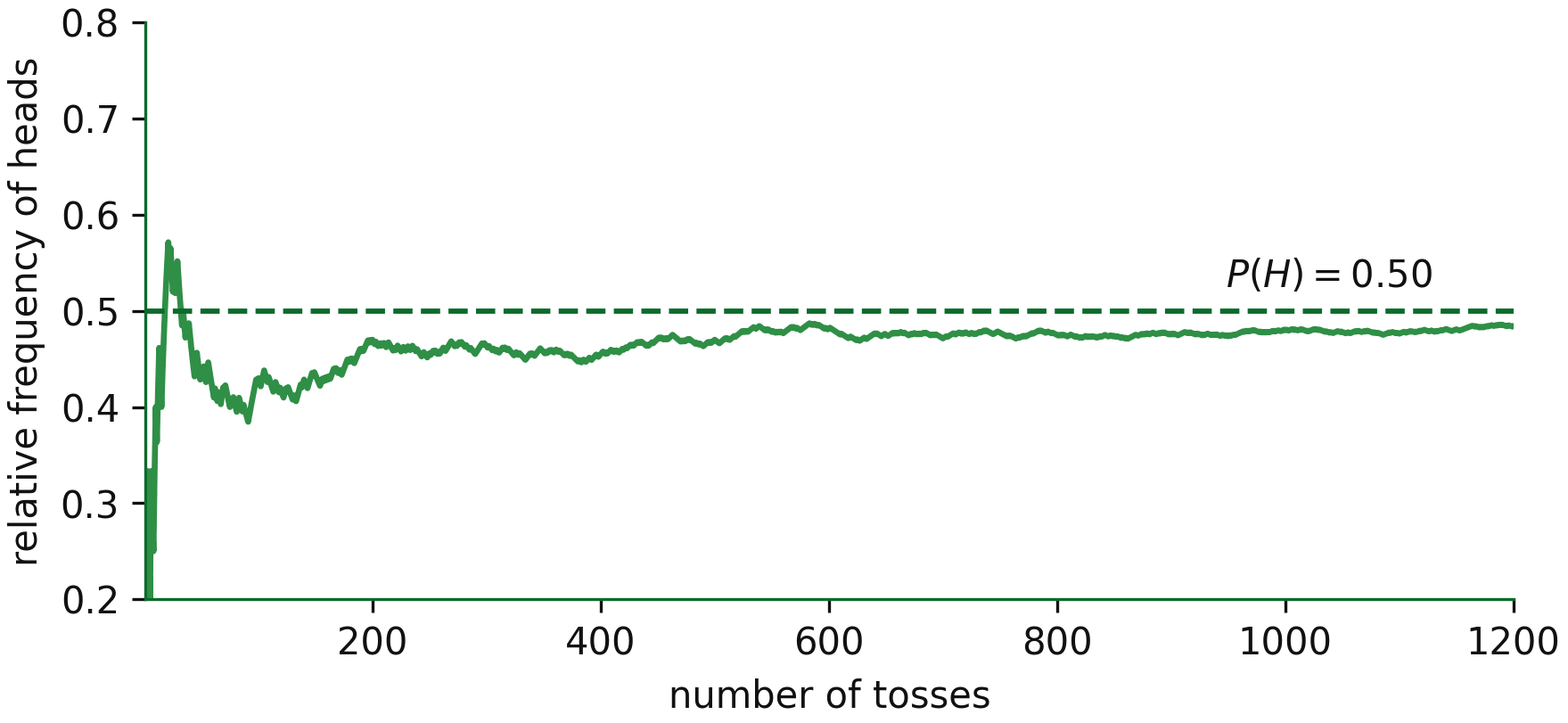
The observed proportion may fluctuate strongly at first. With more repetitions, it typically becomes more stable around the theoretical probability.

1.3.10 Example 4: Toss a Coin 20 Times

Suppose a fair coin is tossed 20 times.

Heads occurs 12 times.

The observed relative frequency of heads is

\[\frac{12}{20}=0.60.\]

For a fair coin, the theoretical probability of heads is

\[P(H)=0.50.\]

Therefore,

\[0.60 \neq 0.50.\]

This does not mean that the coin must be unfair.

With only 20 tosses, random variation can produce more heads or more tails.

For example, a fair coin does not need to produce exactly 10 heads in 20 tosses.

If we repeat the experiment many more times, the relative frequency of heads usually stays closer to \(0.50\).

Note

Theoretical probability and relative frequency may differ when the number of trials is small.

1.3.11 When Outcomes Are Not Equally Likely

The formula

\[P(A)=\frac{n}{N}\]

works only when the outcomes are equally likely.

Sometimes the outcomes have different probabilities.

For example, a loaded die is a die whose faces do not all have the same chance of occurring.

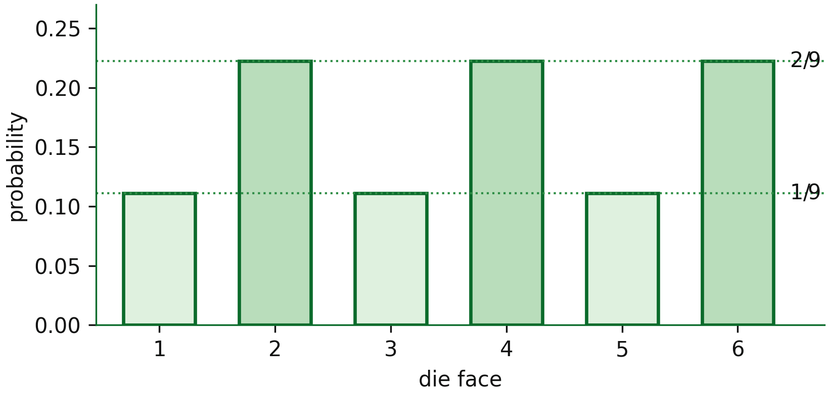
The bars have different heights because the outcomes are not equally likely. In this case, simply counting the number of outcomes is not enough.

Instead, we add the probabilities of the outcomes that belong to the event.

If

\[A=\{a_1,a_2,\ldots,a_k\},\]

then the probability of \(A\) is found by adding the probabilities of those sample points:

\[P(A)=P(a_1)+P(a_2)+\cdots+P(a_k).\]

This is the general idea behind the probability of an event.

1.3.12 Example 5: Loaded Die

Suppose a loaded die has the following probabilities:

• each odd number has probability \(\frac{1}{9}\);

• each even number has probability \(\frac{2}{9}\).

Thus,

\[P(1)=P(3)=P(5)=\frac{1}{9}\]

and

\[P(2)=P(4)=P(6)=\frac{2}{9}.\]

First, notice that the probabilities of all six outcomes add to 1:

\[3\left(\frac{1}{9}\right) + 3\left(\frac{2}{9}\right) = \frac{3}{9}+\frac{6}{9} = 1.\]

Now let

\[D=\{1,2,3\}.\]

To find \(P(D)\), add the probabilities of 1, 2, and 3:

\[P(D) = P(1)+P(2)+P(3).\]

Therefore,

\[P(D) = \frac{1}{9} + \frac{2}{9} + \frac{1}{9} = \frac{4}{9}.\]

The event \(D\) contains 3 of the 6 outcomes, but

\[P(D)\neq\frac{3}{6}.\]

The reason is that the six outcomes are not equally likely.

Note

Use \(P(A)=n/N\) only when outcomes are equally likely.

If outcomes have different probabilities, add the probabilities of the outcomes in \(A\).

1.3.13 A Simple Method

For a basic probability problem, use the following steps.

Step 1: Write the sample space.

Ask:

What are all possible outcomes?

Step 2: Define the event.

Ask:

Which outcomes do we care about?

Step 3: Check whether the outcomes are equally likely.

For example:

• fair coin -> equally likely;

• fair die -> equally likely;

• loaded die -> not equally likely.

Step 4: Choose the correct calculation.

If the outcomes are equally likely, use

\[P(A)=\frac{n}{N}.\]

If the outcomes are not equally likely, add the probabilities of the outcomes in the event.

Step 5: Interpret the answer.

Remember that the final probability must satisfy

\[0\leq P(A)\leq1.\]

For repeated experiments, relative frequency can also be used to describe what was observed.

1.3.14 Common Mistakes

A common mistake is to use the number of favorable outcomes as the probability.

For example, if

\[A=\{5,6\}\]

for one fair die, there are 2 favorable outcomes, but

\[P(A)=\frac{2}{6}=\frac{1}{3},\]

not 2.

Another mistake is to forget that the denominator must count all possible outcomes.

For a fair die, the denominator is 6 because

\[S=\{1,2,3,4,5,6\}.\]

A third mistake is to read at least one as exactly one.

For two coin tosses,

\[\{HH,HT,TH\}\]

represents at least one head.

A fourth mistake is to expect experimental results to match theoretical probability exactly.

A fair coin can produce 12 heads in 20 tosses even though

\[P(H)=0.50.\]

A final mistake is to use

\[P(A)=\frac{n}{N}\]

when the outcomes are not equally likely.

For a loaded die, the probabilities of the individual outcomes must be used.

1.3.15 Summary

Probability tells us how likely an event is to occur.

The main relationship is:

Sample Space -> Event -> Probability

The probability of event \(A\) is written as

\[P(A).\]

Every probability is between 0 and 1:

\[0\leq P(A)\leq1.\]

The impossible event has probability 0:

\[P(\varnothing)=0.\]

The certain event has probability 1:

\[P(S)=1.\]

When all outcomes are equally likely,

\[P(A) = \frac{\text{favorable outcomes}} {\text{total outcomes}} = \frac{n}{N}.\]

Relative frequency is

\[\frac{\text{number of times the event occurs}} {\text{number of trials}}.\]

Relative frequency may differ from theoretical probability in a small number of trials.

When outcomes are not equally likely, add the probabilities of the sample points that belong to the event.

Before calculating a probability:

1. identify the sample space;

2. define the event;

3. check whether the outcomes are equally likely;

4. choose the correct calculation.