3.6 Hypergeometric Distribution

3.6.1 Main Idea

The hypergeometric distribution models the number of items from a group of interest when a sample is selected without replacement from a finite population.

Suppose the population contains

• \(N\) total items;

• \(K\) items in the group of interest;

• \(N-K\) items in the other group.

A sample of size \(n\) is selected without replacement. Define

\[X=\text{number of items from the group of interest in the sample}.\]

The word success is often used for the group being counted. It does not have to mean a desirable outcome. For example, in quality control, a defective item may be called a success if defectives are what \(X\) counts.

A common notation is

\[X\sim\operatorname{Hypergeometric}(N,K,n).\]

Some textbooks instead write the parameters as the size of the first group, the size of the second group, and the sample size. The \(N,K,n\) notation will be used here because it makes the population structure explicit.

3.6.2 Conditions for a Hypergeometric Experiment

A hypergeometric experiment has the following structure:

1. The population is finite and contains two groups.

2. One group is designated as the group of interest.

3. A fixed sample of size \(n\) is selected.

4. Sampling is without replacement.

5. The selections are therefore dependent.

The last point distinguishes a hypergeometric experiment from repeated Bernoulli trials.

A single draw can still be classified as success or failure, but the sequence is not a Bernoulli sequence because the probability of success changes after each draw.

For example, suppose a box contains 4 red and 6 black cards. Initially,

\[P(\text{red on first draw})=\frac4{10}.\]

If the first card is red and is not replaced, then

\[P(\text{red on second draw}\mid\text{first red}) =\frac3{9}.\]

The probability changed because the composition of the population changed.

The figure illustrates the key point: after an item is removed, both the numerator and denominator can change. Thus, later selections depend on the earlier selections.

3.6.3 Parameters and Possible Values

For

\[X\sim\operatorname{Hypergeometric}(N,K,n),\]

we use

• \(N\): population size;

• \(K\): number of successes in the population;

• \(N-K\): number of failures in the population;

• \(n\): sample size;

• \(X\): number of successes in the sample.

The possible values of \(X\) are not always simply \(0,1,\ldots,n\).

The largest possible number of successes is

\[\min(n,K),\]

because we cannot select more successes than the sample size or more than the number available in the population.

The smallest possible number is

\[\max(0,n+K-N).\]

Therefore,

Note

Support of a Hypergeometric Random Variable

\[\max(0,n+K-N) \leq X\leq \min(n,K).\]

For example, if only 10 defective laptops exist in the population, then a sample cannot contain 11 defective laptops even if the sample size is larger than 10.

3.6.4 Deriving the Hypergeometric PMF

Suppose we want exactly \(x\) successes in a sample of size \(n\).

A sample with exactly \(x\) successes must contain

• \(x\) items chosen from the \(K\) successes;

• \(n-x\) items chosen from the \(N-K\) failures.

The number of ways to choose the successes is

\[\binom Kx.\]

The number of ways to choose the failures is

\[\binom{N-K}{n-x}.\]

Therefore, the number of samples having exactly \(x\) successes is

\[\binom Kx\binom{N-K}{n-x}.\]

The total number of samples of size \(n\) that can be selected from \(N\) items is

\[\binom Nn.\]

Because each subset of \(n\) items is equally likely under simple random sampling without replacement,

Note

Hypergeometric PMF

\[P(X=x) = \frac{ \binom Kx \binom{N-K}{n-x} }{ \binom Nn }.\]

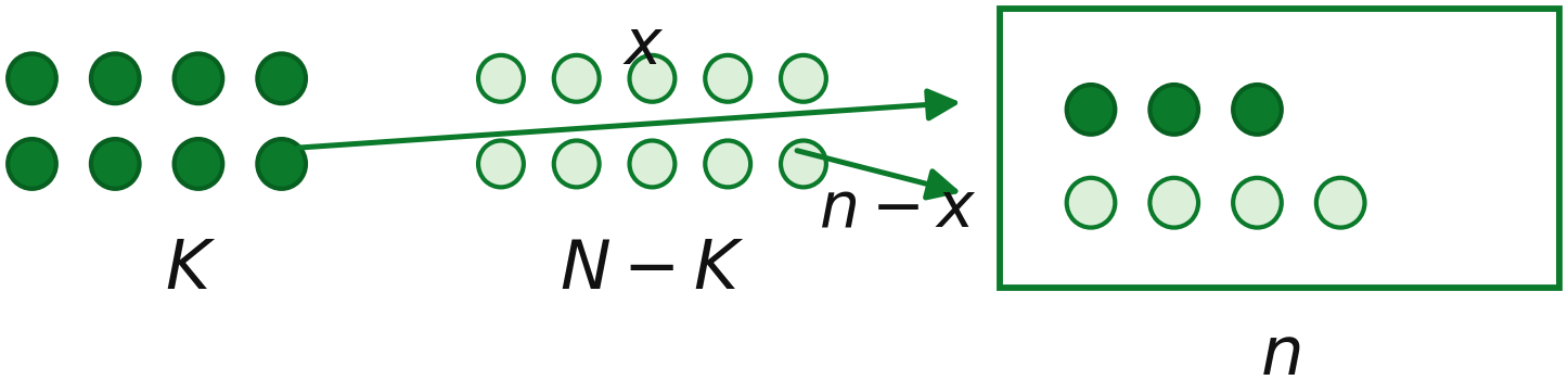
The numerator counts the favorable samples: choose \(x\) objects from the group of interest and \(n-x\) from the other group. The denominator counts all samples of size \(n\).

This is a counting argument rather than a product of independent Bernoulli probabilities.

3.6.5 Example: Inspecting Laptops

A shipment contains 100 laptops, of which 10 are known to be defective. An inspector randomly selects 12 laptops without replacement.

Let

\[X=\text{number of defective laptops in the sample}.\]

Then

\[N=100, \qquad K=10, \qquad n=12.\]

The possible values are

\[X=0,1,2,\ldots,10.\]

The upper limit is 10, not 12, because only 10 defective laptops exist in the entire shipment.

Suppose we want the probability that at most two sampled laptops are defective:

\[P(X\leq2) = P(X=0)+P(X=1)+P(X=2).\]

Using the hypergeometric PMF,

\[P(X\leq2) = \sum_{x=0}^{2} \frac{ \binom{10}{x} \binom{90}{12-x} }{ \binom{100}{12} }.\]

The three probabilities are approximately

\[P(X=0)=0.2608, \qquad P(X=1)=0.3961, \qquad P(X=2)=0.2451.\]

Therefore,

\[P(X\leq2) \approx 0.2608+0.3961+0.2451 =0.9019.\]

Thus, there is about a \(90.19\%\) probability that the sample contains at most two defective laptops.

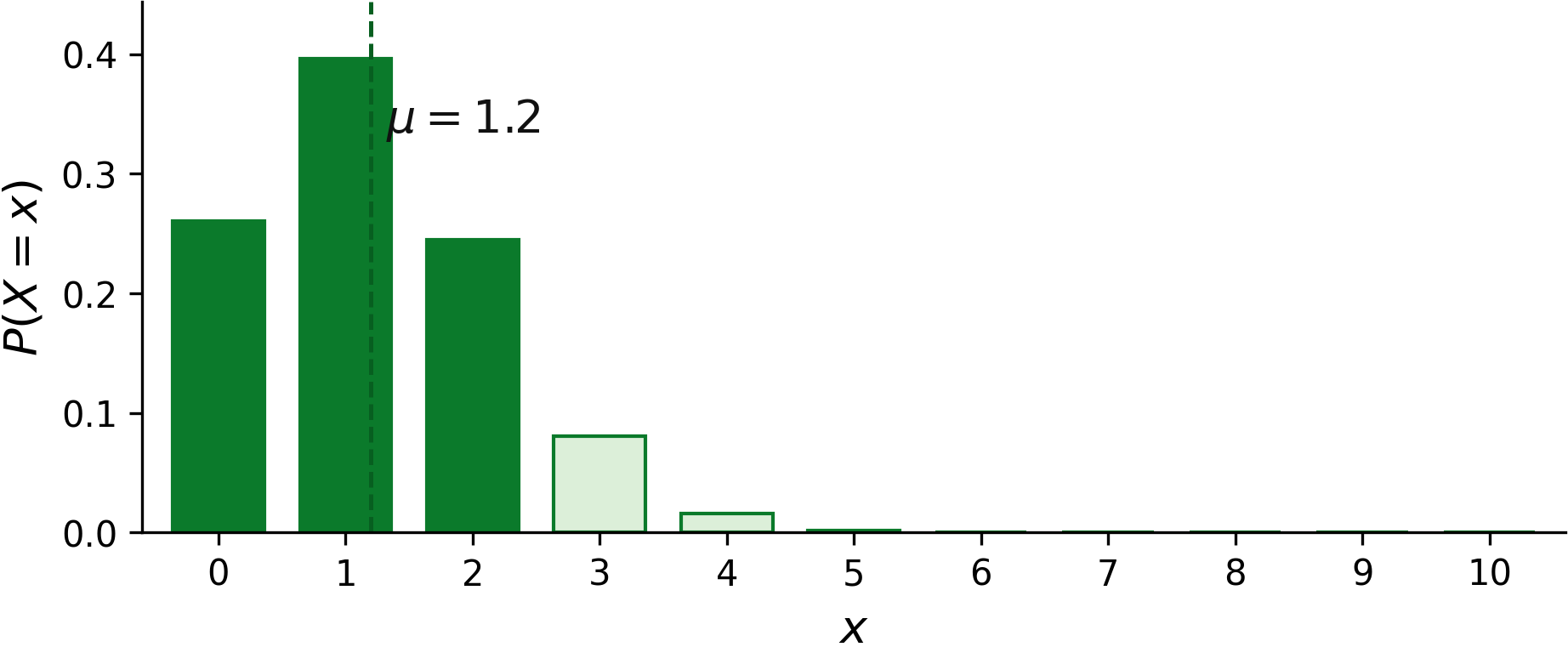
The darker bars represent the event \(X\leq2\). The distribution is centered near \(1.2\), the expected number of defectives in a sample of 12.

3.6.6 Deriving the Mean

The mean has a simple form even though the draws are dependent.

For draw \(i\), define the indicator variable

\[\begin{split}I_i= \begin{cases} 1, & \text{if draw }i\text{ is a success},\\ 0, & \text{otherwise}. \end{cases}\end{split}\]

The total number of successes is

\[X=I_1+I_2+\cdots+I_n.\]

Before any particular draw position is observed, every population item is equally likely to occupy that position. Therefore,

\[P(I_i=1)=\frac KN.\]

Hence,

\[E(I_i)=\frac KN.\]

Using linearity of expectation,

\[E(X) = E(I_1)+\cdots+E(I_n) = n\frac KN.\]

Thus,

Note

Mean of a Hypergeometric Distribution

\[\boxed{ E(X)=n\frac KN }\]

If we define the population success proportion as

\[p=\frac KN,\]

then the same result is

\[E(X)=np.\]

Notice that this has the same form as the binomial mean.

For the laptop example,

\[E(X) = 12\left(\frac{10}{100}\right) =1.2.\]

An expected value of 1.2 does not mean that a sample can contain 1.2 defective laptops. It is the long-run average number of defectives over many samples.

3.6.7 Deriving the Variance

The variance differs from the binomial variance because the draws are not independent.

Let

\[p=\frac KN, \qquad q=1-p.\]

For each indicator \(I_i\),

\[\operatorname{Var}(I_i)=pq.\]

For two different draw positions \(i\) and \(j\),

\[P(I_i=1,I_j=1) = \frac KN \frac{K-1}{N-1}.\]

Therefore,

\[\operatorname{Cov}(I_i,I_j) = P(I_i=1,I_j=1)-p^2.\]

Substituting gives

\[\operatorname{Cov}(I_i,I_j) = \frac KN\frac{K-1}{N-1} - \left(\frac KN\right)^2.\]

After simplifying,

\[\operatorname{Cov}(I_i,I_j) = -\frac{p(1-p)}{N-1} = -\frac{pq}{N-1}.\]

The covariance is negative: if one draw is a success, there is one fewer success available for a later draw.

Now

\[X=\sum_{i=1}^{n}I_i,\]

so

\[\operatorname{Var}(X) = \sum_{i=1}^{n}\operatorname{Var}(I_i) + 2\sum_{i<j}\operatorname{Cov}(I_i,I_j).\]

There are \(n\) variance terms and \(\binom n2\) covariance pairs. Thus,

\[\operatorname{Var}(X) = npq + 2\binom n2 \left(-\frac{pq}{N-1}\right).\]

Since

\[2\binom n2=n(n-1),\]

we obtain

\[\operatorname{Var}(X) = npq - \frac{n(n-1)pq}{N-1}.\]

Factor \(npq\):

\[\operatorname{Var}(X) = npq \left[ 1-\frac{n-1}{N-1} \right].\]

Therefore,

Note

Variance of a Hypergeometric Distribution

\[\boxed{ \operatorname{Var}(X) = np(1-p) \left(\frac{N-n}{N-1}\right) }\]

The factor

\[\frac{N-n}{N-1}\]

is the finite population correction. It reduces the variance because sampling without replacement creates negative dependence.

The standard deviation is

\[\sigma = \sqrt{ np(1-p) \left(\frac{N-n}{N-1}\right) }.\]

For the laptop example,

\[p=\frac{10}{100}=0.10.\]

Thus,

\[\operatorname{Var}(X) = 12(0.10)(0.90) \left(\frac{100-12}{100-1}\right) =0.96,\]

and

\[\sigma = \sqrt{0.96} \approx0.980.\]

3.6.8 Probability Language and the CDF

As with other discrete distributions, probability statements should first be translated into events involving \(X\).

Exactly two means

\[P(X=2).\]

At most two means

\[P(X\leq2).\]

At least two means

\[P(X\geq2).\]

The hypergeometric CDF is obtained by summing PMF values:

\[F(x) = P(X\leq x) = \sum_{j=x_{\min}}^{x} \frac{ \binom Kj \binom{N-K}{n-j} }{ \binom Nn }.\]

There is no need to memorize a separate closed-form expression. The important idea is that cumulative probabilities are sums of hypergeometric PMF values.

Complements are often convenient. For example,

\[P(X\geq1) = 1-P(X=0).\]

3.6.9 Hypergeometric Versus Binomial

The random variable may look the same in both models: both can count the number of successes in a sample. The sampling mechanism determines the model.

Feature	Binomial	Hypergeometric
Number sampled	Fixed \(n\)	Fixed \(n\)
Outcomes per draw	Two categories	Two categories
Replacement	With replacement or effectively unchanged	Without replacement
Success probability	Constant \(p\)	Changes across draws
Draws	Independent	Dependent
Random variable	Number of successes	Number of successes

The two means have the same form,

\[E(X)=np,\]

but the variances differ:

\[\operatorname{Var}_{\text{Binomial}}(X) =np(1-p),\]

whereas

\[\operatorname{Var}_{\text{Hypergeometric}}(X) = np(1-p) \left(\frac{N-n}{N-1}\right).\]

Because

\[\frac{N-n}{N-1}<1\]

when \(n>1\), the hypergeometric distribution is less variable than the corresponding binomial distribution with the same \(n\) and \(p\).

3.6.10 Binomial Approximation

If the population is very large relative to the sample, removing one item has only a small effect on the success probability.

In that situation, the hypergeometric distribution can sometimes be approximated by

\[Y\sim\operatorname{Binomial} \left(n,\frac KN\right).\]

A common introductory rule of thumb is

\[\frac nN\leq0.05.\]

When the sampling fraction is small, the finite population correction is close to 1, so the hypergeometric and binomial variances are also close.

This is an approximation, not an exact equality.

3.6.11 Example: Selecting a Committee

A committee of four is selected randomly from six men and five women. Let

\[X=\text{number of men on the committee}.\]

Then

\[N=11, \qquad K=6, \qquad n=4.\]

The probability that exactly two committee members are men is

\[P(X=2) = \frac{ \binom62\binom52 }{ \binom{11}{4} }.\]

Therefore,

\[P(X=2) = \frac{15(10)}{330} = \frac{150}{330} \approx0.4545.\]

The expected number of men is

\[E(X) = 4\left(\frac6{11}\right) = \frac{24}{11} \approx2.18.\]

3.6.12 A Simple Modeling Procedure

For a possible hypergeometric problem:

1. Identify the finite population.

2. Confirm that sampling is without replacement.

3. Define the group of interest as success.

4. Identify \(N\), \(K\), and \(n\).

5. Define \(X\) as the number of successes in the sample.

6. Determine the valid range of \(X\).

7. Translate the requested probability into notation.

8. Apply the hypergeometric PMF or sum PMF values as needed.

3.6.13 Common Mistakes

Do not use a binomial model merely because the problem counts successes. Check whether sampling is without replacement from a finite population.

Do not treat the draws as independent. The population composition changes after every selection.

Do not confuse \(N\) and \(n\):

• \(N\) is the population size;

• \(n\) is the sample size.

Do not forget that the number of failures in the population is

\[N-K.\]

Do not assume that \(X\) always ranges from \(0\) to \(n\). Use

\[\max(0,n+K-N) \leq X\leq \min(n,K).\]

3.6.14 Summary

The hypergeometric distribution models the number of successes in a fixed-size sample selected without replacement from a finite population.

For

\[X\sim\operatorname{Hypergeometric}(N,K,n),\]

its PMF is

\[P(X=x) = \frac{ \binom Kx \binom{N-K}{n-x} }{ \binom Nn }.\]

The mean is

\[E(X)=n\frac KN.\]

The variance is

\[\operatorname{Var}(X) = np(1-p) \left(\frac{N-n}{N-1}\right), \qquad p=\frac KN.\]

The key modeling question is:

Is the sample taken without replacement from a finite population?

If yes, the hypergeometric distribution should be considered before the binomial distribution.