3.2 Discrete Uniform Distribution

3.2.1 Main Idea

The discrete uniform distribution applies when a random variable has a finite number of possible values and every value is equally likely.

Suppose

\[X\in\{x_1,x_2,\ldots,x_n\}\]

and all \(n\) values are equally likely. Then

Note

Discrete Uniform Distribution

\[P(X=x_i)=\frac{1}{n}, \qquad i=1,2,\ldots,n.\]

The word uniform means that the probability is distributed equally over all possible values.

A discrete uniform PMF therefore has the same probability height at every allowed value. The possible values remain separate points, but none is more likely than another.

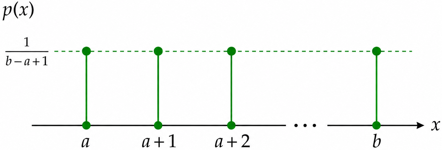
In the figure, each possible value receives the same probability \(1/(b-a+1)\). This equal-height pattern is the defining graphical feature of a discrete uniform distribution.

3.2.2 Example 1: Random Digit

Suppose one digit is selected at random from

\[\{0,1,2,\ldots,9\}.\]

Let \(X\) be the selected digit. There are

\[n=10\]

possible values and each is equally likely, so

\[P(X=x)=\frac{1}{10}, \qquad x=0,1,\ldots,9.\]

The PMF therefore has the same height at every possible value.

3.2.3 Consecutive Integer Values

A common discrete uniform model uses consecutive integers

\[a,a+1,\ldots,b.\]

The number of possible values is

\[n=b-a+1.\]

Therefore,

\[P(X=x) = \frac{1}{n} = \frac{1}{b-a+1}, \qquad x=a,a+1,\ldots,b.\]

The formulas for the mean and variance can be derived directly from this PMF.

3.2.4 Deriving the Mean

For any discrete random variable,

\[E(X)=\sum_x x\,p(x).\]

For a discrete uniform random variable on \(\{a,a+1,\ldots,b\}\), every value has probability \(1/n\). Therefore,

\[E(X) = \sum_{x=a}^{b}x\left(\frac1n\right) = \frac1n\sum_{x=a}^{b}x.\]

To evaluate the sum, recall

\[1+2+\cdots+m = \frac{m(m+1)}{2}.\]

Hence,

\[\sum_{x=a}^{b}x = \left(1+2+\cdots+b\right) - \left(1+2+\cdots+(a-1)\right).\]

Using the sum-of-integers identity,

\[\sum_{x=a}^{b}x = \frac{b(b+1)}{2} - \frac{(a-1)a}{2}.\]

Substitute this into the expectation:

\[E(X) = \frac1n \left[ \frac{b(b+1)-(a-1)a}{2} \right].\]

Expand the numerator:

\[b(b+1)-(a-1)a = b^2+b-a^2+a.\]

Factor:

\[b^2+b-a^2+a = (a+b)(b-a+1).\]

Because

\[n=b-a+1,\]

we obtain

\[E(X) = \frac{(a+b)n}{2n} = \frac{a+b}{2}.\]

Thus,

Note

Mean of a Discrete Uniform Distribution

\[\boxed{E(X)=\mu=\frac{a+b}{2}}.\]

The mean is halfway between the smallest and largest possible values. This can also be interpreted as a balance point. Because all values carry equal probability weight, the loading is symmetric around the midpoint.

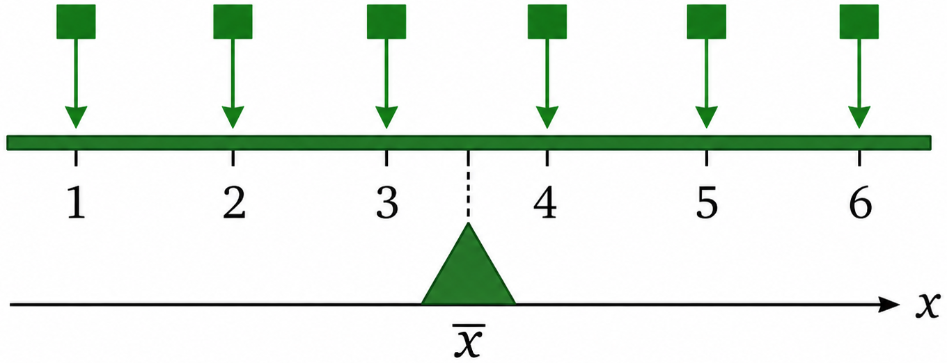
For a fair die, the equal probability weights at \(1,2,3,4,5,6\) balance at \(3.5\). The expected value does not need to be one of the possible outcomes; it represents the center of the probability loading.

3.2.5 Deriving the Variance

For a discrete random variable,

\[\operatorname{Var}(X) = E(X^2)-[E(X)]^2.\]

We already know

\[E(X)=\frac{a+b}{2}.\]

Therefore, we first derive \(E(X^2)\).

Because every value has probability \(1/n\),

\[E(X^2) = \sum_{x=a}^{b}x^2\left(\frac1n\right) = \frac1n\sum_{x=a}^{b}x^2.\]

Recall the sum-of-squares identity

\[1^2+2^2+\cdots+m^2 = \frac{m(m+1)(2m+1)}{6}.\]

Therefore,

\[\sum_{x=a}^{b}x^2 = \left(1^2+2^2+\cdots+b^2\right) - \left(1^2+2^2+\cdots+(a-1)^2\right).\]

Applying the identity gives

\[\sum_{x=a}^{b}x^2 = \frac{b(b+1)(2b+1)}{6} - \frac{(a-1)a(2a-1)}{6}.\]

Hence,

\[E(X^2) = \frac{1}{6n} \left[ b(b+1)(2b+1) - (a-1)a(2a-1) \right].\]

Now substitute \(E(X^2)\) and \(E(X)=(a+b)/2\) into the variance formula:

\[\operatorname{Var}(X) = \frac{1}{6n} \left[ b(b+1)(2b+1) - (a-1)a(2a-1) \right] - \left(\frac{a+b}{2}\right)^2.\]

Using \(n=b-a+1\) and simplifying the algebra gives

\[\operatorname{Var}(X) = \frac{(b-a+1)^2-1}{12}.\]

Since \(n=b-a+1\), this can also be written as

\[\operatorname{Var}(X) = \frac{n^2-1}{12}.\]

Thus,

Note

Variance and Standard Deviation

\[\boxed{ \operatorname{Var}(X) = \frac{(b-a+1)^2-1}{12} = \frac{n^2-1}{12} }\]

and

\[\boxed{ \sigma = \sqrt{\operatorname{Var}(X)} }.\]

3.2.6 Example 2: Rolling a Fair Die

Roll one fair six-sided die and let

\[X=\text{number shown}.\]

Then

\[X\in\{1,2,3,4,5,6\},\]

so

\[a=1, \qquad b=6, \qquad n=b-a+1=6.\]

Each value has probability

\[P(X=x)=\frac16.\]

The PMF is flat because every die face is equally likely.

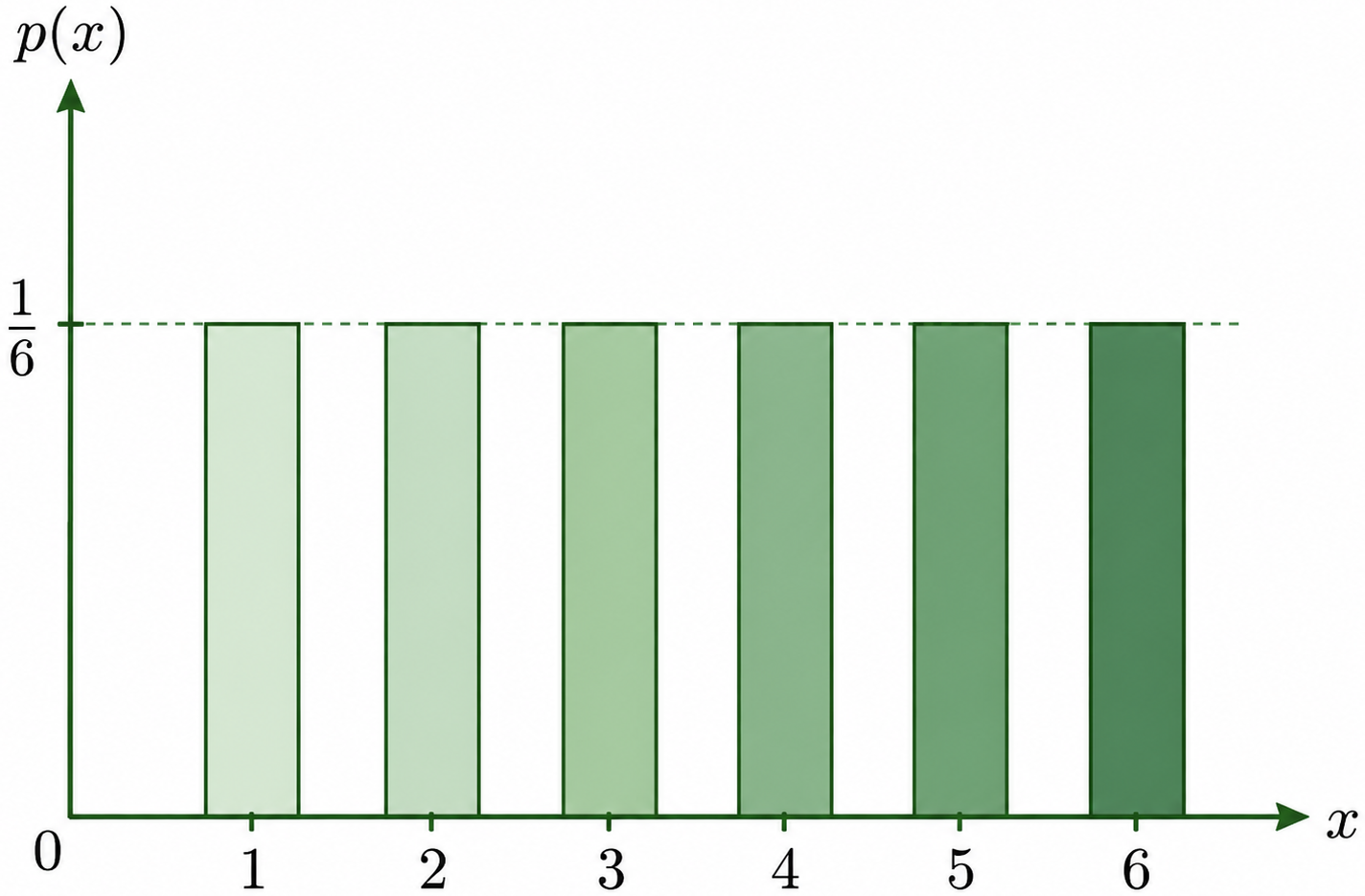
The six equal bars make the uniform assumption visible: changing the value of \(x\) from 1 to 6 does not change \(P(X=x)\).

Mean

Using the discrete-uniform mean formula,

\[E(X) = \frac{a+b}{2} = \frac{1+6}{2} = \frac72 = 3.5.\]

The same result can be checked directly from the PMF:

\[E(X) = \sum_{x=1}^{6}x\left(\frac16\right) = \frac{1+2+3+4+5+6}{6} = \frac{21}{6} = 3.5.\]

Variance

Using \(n=6\),

\[\operatorname{Var}(X) = \frac{n^2-1}{12} = \frac{6^2-1}{12} = \frac{36-1}{12} = \frac{35}{12} \approx 2.917.\]

The same result can also be obtained from \(E(X^2)-[E(X)]^2\):

\[E(X^2) = \frac{1^2+2^2+3^2+4^2+5^2+6^2}{6} = \frac{91}{6}.\]

Therefore,

\[\operatorname{Var}(X) = \frac{91}{6} - \left(\frac72\right)^2 = \frac{182}{12} - \frac{147}{12} = \frac{35}{12}.\]

Standard deviation

\[\sigma = \sqrt{\frac{35}{12}} \approx 1.708.\]

The expected outcome is 3.5. The standard deviation indicates that outcomes typically vary from this center by about 1.71 units.

For example,

\[P(X\geq5) = P(X=5)+P(X=6) = \frac16+\frac16 = \frac13.\]

3.2.7 When Should We Use It?

Use a discrete uniform model when:

• there is a finite set of possible values;

• each possible value has the same probability.

Typical examples include:

• one fair die;

• a randomly selected digit;

• a randomly selected numbered tag;

• one randomly selected integer from a specified finite set.

Do not use a discrete uniform distribution merely because the possible values are equally spaced.

Equal spacing does not imply equal probability.

3.2.8 Quick Practice

A box contains five tags labeled

\[2,3,4,5,6.\]

One tag is selected at random and each tag is equally likely. Let \(X\) be the number on the selected tag.

Find:

1. \(P(X=4)\);

2. \(P(X>4)\);

3. \(E(X)\); and

4. \(\operatorname{Var}(X)\).

Answer

There are five equally likely values, so

\[P(X=4)=\frac15.\]

For \(X>4\), the favorable values are 5 and 6:

\[P(X>4)=\frac25.\]

Here,

\[a=2, \qquad b=6, \qquad n=5.\]

Thus,

\[E(X) = \frac{2+6}{2} = 4,\]

and

\[\operatorname{Var}(X) = \frac{5^2-1}{12} = 2.\]

3.2.9 Common Mistakes

A common mistake is to assume that every discrete variable is uniform.

For two coin tosses, the number of heads has possible values \(0,1,2\), but their probabilities are not equal.

Another mistake is to count the integers from \(a\) through \(b\) as \(b-a\). Because both endpoints are included, the correct number is

\[n=b-a+1.\]

When deriving the variance, do not forget that

\[\operatorname{Var}(X) = E(X^2)-[E(X)]^2,\]

not \(E(X^2)-E(X)\).

3.2.10 Summary

For a discrete uniform random variable on the consecutive integers

\[a,a+1,\ldots,b,\]

there are

\[n=b-a+1\]

possible values, each with probability

\[P(X=x)=\frac1n.\]

The mean is

\[E(X)=\frac{a+b}{2}.\]

The variance is

\[\operatorname{Var}(X) = \frac{n^2-1}{12} = \frac{(b-a+1)^2-1}{12}.\]

The standard deviation is

\[\sigma = \sqrt{\operatorname{Var}(X)}.\]

The key modeling question is:

Are all possible values equally likely?