3.4 Geometric Distribution

Key Terms

Geometric distribution（幾何分配）

A discrete distribution for the number of independent Bernoulli trials required to obtain the first success.

Waiting time（等待次數）

The number of trials required before a specified success occurs.

Memoryless property（無記憶性）

After any number of failures, the future waiting distribution is the same as it was at the beginning.

3.4.1 Main Idea

The geometric distribution uses the same Bernoulli-trial structure as the binomial distribution:

• each trial has two outcomes, success or failure;

• trials are independent;

• the probability of success \(p\) is constant;

• the probability of failure is \(q=1-p\).

The difference is the stopping rule.

For a binomial experiment, the number of trials is fixed and we count successes. For a geometric experiment, we repeat trials until the first success and count how many trials are required.

Let

\[X=\text{trial number on which the first success occurs}.\]

Then

\[X\in\{1,2,3,\ldots\}.\]

The number of possible trials is not fixed in advance. In principle, the waiting time can be arbitrarily large.

3.4.2 Bernoulli-Trial Structure

A geometric experiment is built from repeated Bernoulli trials. Every trial must have the same success probability \(p\) and failure probability \(q=1-p\).

The experiment stops as soon as the first success occurs. For example, if the first success occurs on trial 4, the observed sequence must have the form

\[F,F,F,S.\]

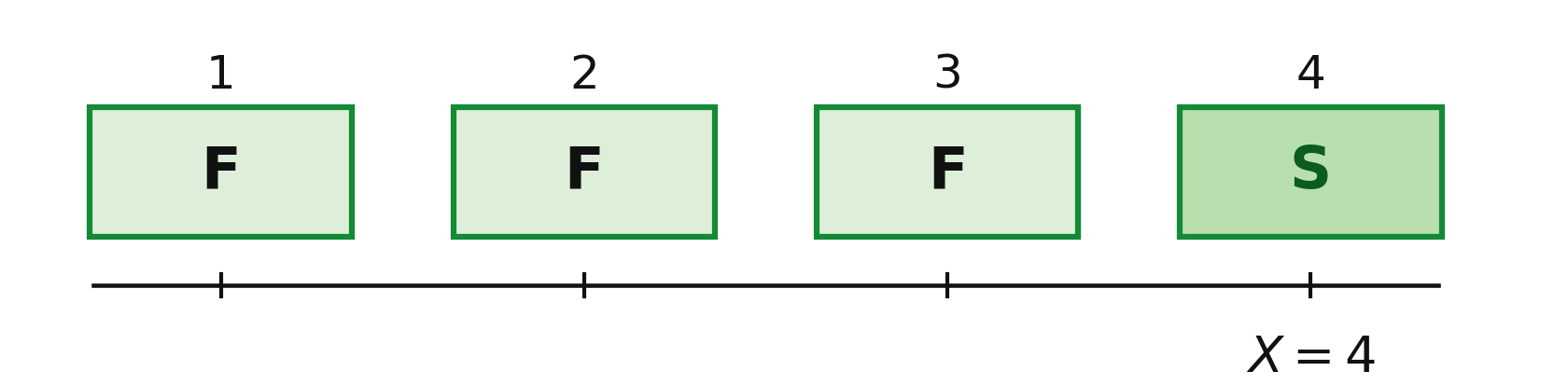
The first three trials are failures and the fourth trial is the first success. This failure-then-success structure is the key to the geometric PMF.

3.4.3 Two Common Random-Variable Conventions

There are two common ways to define a geometric random variable. The formulas look slightly different, so the definition of the random variable must always be checked first.

In this handout, the main convention is

\[X=\text{number of trials until and including the first success}.\]

Thus,

\[X=1,2,3,\ldots.\]

An alternative convention is

\[Y=\text{number of failures before the first success}.\]

Then

\[Y=0,1,2,\ldots\]

and the two variables are related by

\[Y=X-1.\]

Unless stated otherwise, the remainder of this section uses \(X\), the trial number of the first success.

3.4.4 Deriving the Geometric PMF

Suppose the first success occurs on trial \(x\).

Then the first \(x-1\) trials must all be failures, followed by a success on trial \(x\):

\[\underbrace{F\,F\,\cdots\,F}_{x-1\text{ failures}}\,S.\]

Because the trials are independent,

\[P(\text{first }x-1\text{ trials fail}) =q^{x-1}.\]

The probability that trial \(x\) is a success is \(p\). Therefore, by the multiplication rule,

\[P(X=x) =q^{x-1}p.\]

Since \(q=1-p\), we obtain

Note

Geometric PMF

\[\boxed{ P(X=x)=(1-p)^{x-1}p, \qquad x=1,2,3,\ldots }\]

Unlike a binomial PMF, there is no combination coefficient. Once \(x\) is specified, the order is fixed: all previous trials must be failures and the last trial must be the first success.

3.4.5 Why the PMF Sums to 1

Let \(q=1-p\). Then

\[\sum_{x=1}^{\infty}P(X=x) = \sum_{x=1}^{\infty}q^{x-1}p.\]

Factor out \(p\):

\[\sum_{x=1}^{\infty}P(X=x) = p\sum_{x=1}^{\infty}q^{x-1}.\]

Using the geometric-series identity

\[1+q+q^2+\cdots = \frac{1}{1-q}, \qquad |q|<1,\]

we obtain

\[\sum_{x=1}^{\infty}P(X=x) = p\left(\frac{1}{1-q}\right).\]

Because \(1-q=p\),

\[\sum_{x=1}^{\infty}P(X=x)=1.\]

Thus the geometric PMF is a valid probability distribution.

3.4.6 Why It Is Called “Geometric”

Successive probabilities form a geometric sequence. In fact,

\[\frac{P(X=x+1)}{P(X=x)} = \frac{q^x p}{q^{x-1}p} =q.\]

Therefore,

\[P(X=x+1)=qP(X=x).\]

Each bar is a constant fraction \(q=1-p\) of the previous bar.

For example, when \(p=0.25\), the probabilities decrease by the common ratio \(q=0.75\).

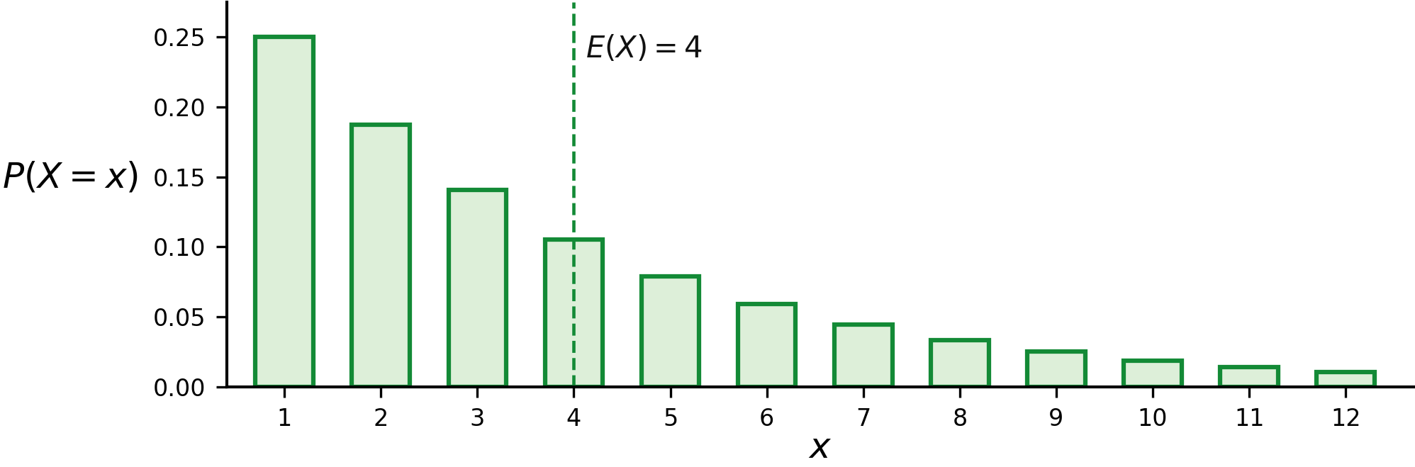
The distribution is right-skewed: small waiting times are most likely, while large waiting times remain possible but become progressively less probable.

3.4.7 Example: First Success with \(p=0.25\)

Suppose independent Bernoulli trials have

\[p=0.25, \qquad q=0.75.\]

Let \(X\) be the number of trials until the first success.

To find the probability that the first success occurs on trial 4,

\[P(X=4) =q^3p =(0.75)^3(0.25).\]

Therefore,

\[P(X=4) =0.10546875 \approx0.1055.\]

The event requires exactly three failures followed by one success.

3.4.8 CDF and Tail Probabilities

The event \(X>x\) means that the first \(x\) trials are all failures. Therefore,

\[\boxed{P(X>x)=q^x=(1-p)^x}.\]

The cumulative distribution function follows from the complement rule:

\[F(x) =P(X\le x) =1-P(X>x).\]

Thus, for positive integers \(x\),

Note

Geometric CDF

\[\boxed{F(x)=1-(1-p)^x}.\]

Closely related forms are

\[P(X\ge k)=q^{k-1}\]

and

\[P(X<k)=1-q^{k-1}.\]

For \(p=0.25\),

\[P(X>3) =(0.75)^3 =0.421875.\]

Equivalently, there is a 42.19% chance that the first three trials all fail.

3.4.9 Memoryless Property

The geometric distribution is memoryless. If no success has occurred in the first \(k\) trials, the future waiting-time distribution is the same as if the experiment had just started.

For integers \(k,m\ge0\),

\[P(X>k+m\mid X>k) = \frac{P(X>k+m)}{P(X>k)}.\]

Using the tail formula,

\[P(X>k+m\mid X>k) = \frac{q^{k+m}}{q^k} =q^m.\]

But

\[P(X>m)=q^m.\]

Therefore,

Note

Memoryless Property

\[\boxed{ P(X>k+m\mid X>k)=P(X>m) }.\]

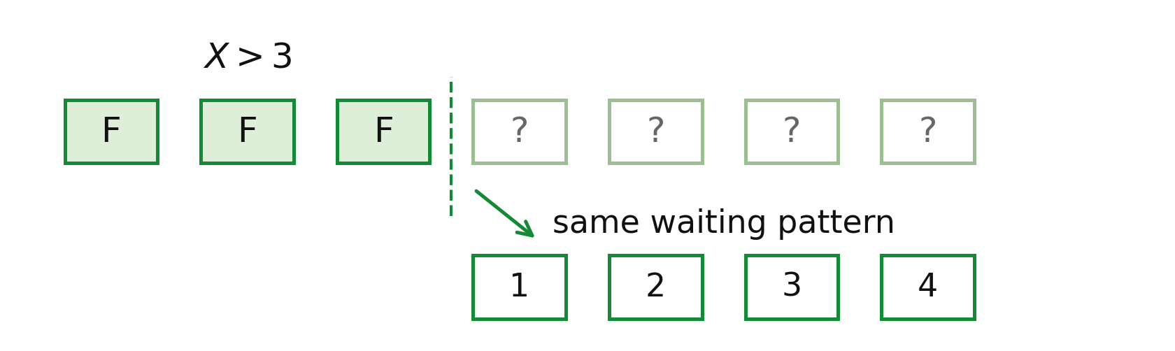
Previous failures do not make a success “due.” The property follows from the independence of the Bernoulli trials and the fact that \(p\) remains constant.

For example, if \(p=0.25\) and the first five trials have failed, then

\[P(\text{more than 3 additional trials}\mid\text{first 5 failed}) =(0.75)^3.\]

This is exactly the same probability as needing more than 3 trials from a fresh start.

3.4.10 Deriving the Mean

For a geometric random variable,

\[E(X) = \sum_{x=1}^{\infty}xP(X=x).\]

Substitute the PMF:

\[E(X) = p\sum_{x=1}^{\infty}xq^{x-1}.\]

Start from the geometric series

\[\sum_{x=0}^{\infty}q^x = \frac{1}{1-q}.\]

Differentiate both sides with respect to \(q\):

\[\sum_{x=1}^{\infty}xq^{x-1} = \frac{1}{(1-q)^2}.\]

Therefore,

\[E(X) = p\left(\frac{1}{(1-q)^2}\right).\]

Since \(1-q=p\),

\[E(X) = \frac{p}{p^2} = \frac1p.\]

Thus,

Note

Mean of a Geometric Distribution

\[\boxed{E(X)=\frac1p}.\]

For \(p=0.25\),

\[E(X)=\frac1{0.25}=4.\]

Over many repetitions, the first success occurs after 4 trials on average. The mean need not be an integer even though \(X\) takes only integer values.

3.4.11 Deriving the Variance

Use

\[\operatorname{Var}(X) = E(X^2)-[E(X)]^2.\]

First,

\[E(X^2) = p\sum_{x=1}^{\infty}x^2q^{x-1}.\]

From the geometric series,

\[\sum_{x=1}^{\infty}xq^x = \frac{q}{(1-q)^2}.\]

Differentiate again:

\[\sum_{x=1}^{\infty}x^2q^{x-1} = \frac{1+q}{(1-q)^3}.\]

Hence,

\[E(X^2) = p\frac{1+q}{(1-q)^3}.\]

Since \(1-q=p\),

\[E(X^2) = \frac{1+q}{p^2}.\]

Now subtract the squared mean:

\[\operatorname{Var}(X) = \frac{1+q}{p^2} - \left(\frac1p\right)^2.\]

Therefore,

\[\operatorname{Var}(X) = \frac{q}{p^2} = \frac{1-p}{p^2}.\]

Thus,

Note

Variance and Standard Deviation

\[\boxed{ \operatorname{Var}(X)=\frac{1-p}{p^2} }\]

and

\[\boxed{ \sigma=\frac{\sqrt{1-p}}{p} }.\]

For \(p=0.25\),

\[\operatorname{Var}(X) = \frac{0.75}{(0.25)^2} =12,\]

so

\[\sigma=\sqrt{12}\approx3.464.\]

3.4.12 Alternative Convention: Failures Before Success

Suppose instead that

\[Y=\text{number of failures before the first success}.\]

Then \(Y=X-1\), so

\[Y\in\{0,1,2,\ldots\}.\]

Its PMF is

\[P(Y=y)=q^yp, \qquad y=0,1,2,\ldots.\]

Because \(Y=X-1\),

\[E(Y) =E(X)-1 =\frac1p-1 =\frac{1-p}{p},\]

while subtracting a constant does not change variance:

\[\operatorname{Var}(Y) = \operatorname{Var}(X) = \frac{1-p}{p^2}.\]

This convention explains why geometric formulas may appear different across textbooks or software packages. Always check what the random variable counts.

3.4.13 Geometric as a Special Negative Binomial Case

The negative binomial distribution counts the number of trials required to obtain the \(r\)-th success. Setting

\[r=1\]

means stopping at the first success. Therefore, the geometric distribution is the special negative binomial case \(r=1\).

The negative-binomial PMF

\[P(X=x) = \binom{x-1}{r-1}p^r(1-p)^{x-r}\]

becomes

\[P(X=x) = \binom{x-1}{0}p(1-p)^{x-1} = p(1-p)^{x-1}.\]

3.4.14 Binomial Versus Geometric

Feature	Binomial	Geometric
Number of trials	Fixed \(n\)	Random
Number of successes	Random	Stop at first success
Random variable	Number of successes	Trials until first success
Support	\(0,1,\ldots,n\)	\(1,2,3,\ldots\)
Main question	How many successes?	How long until success?

The modeling distinction is more important than memorizing formulas.

3.4.15 A Simple Method

For a possible geometric problem:

1. Define what counts as a success.

2. Verify independent Bernoulli trials.

3. Verify that \(p\) is constant.

4. Check that trials continue until the first success.

5. Define clearly whether the random variable counts trials or failures.

6. Translate the requested event before calculating.

7. Use the PMF, CDF, or tail formula as appropriate.

3.4.16 Quick Practice

A fair six-sided die is rolled repeatedly. Define success as rolling a 6. Let \(X\) be the number of rolls until the first 6.

Find:

1. \(P(X=3)\);

2. \(P(X>3)\);

3. \(E(X)\); and

4. \(\operatorname{Var}(X)\).

Answer

Here,

\[p=\frac16, \qquad q=\frac56.\]

Therefore,

\[P(X=3) = \left(\frac56\right)^2\left(\frac16\right) = \frac{25}{216}.\]

Also,

\[P(X>3) = \left(\frac56\right)^3 = \frac{125}{216}.\]

The mean is

\[E(X)=\frac1p=6,\]

and the variance is

\[\operatorname{Var}(X) = \frac{1-p}{p^2} = \frac{5/6}{(1/6)^2} =30.\]

3.4.17 Common Mistakes

Do not use \(q^xp\) when \(X\) counts the trial number of the first success. There are only \(x-1\) failures before trial \(x\).

Do not include \(X=0\) under the trial-count convention. At least one trial is required.

Do not confuse “trials until first success” with “failures before first success.” They differ by 1.

Do not use a geometric model if \(p\) changes from trial to trial. For example, learning, fatigue, or sampling without replacement can violate the constant-probability assumption.

Do not interpret a long run of failures as evidence that success is now more likely. Under the geometric assumptions, the process is memoryless.

3.4.18 Summary

For

\[X=\text{number of trials until the first success},\]

with independent Bernoulli trials and constant success probability \(p\),

\[P(X=x) = (1-p)^{x-1}p, \qquad x=1,2,3,\ldots.\]

The CDF and tail probability are

\[P(X\le x)=1-(1-p)^x\]

and

\[P(X>x)=(1-p)^x.\]

The mean and variance are

\[E(X)=\frac1p\]

and

\[\operatorname{Var}(X)=\frac{1-p}{p^2}.\]

The key modeling question is:

Are we counting a fixed number of successes, or waiting until the first success occurs?