3.5 Negative Binomial Distribution

Key Terms

Negative binomial distribution（負二項分配）

A distribution for the number of Bernoulli trials required to obtain a fixed number of successes.

Required successes（目標成功次數）

The fixed number \(r\) of successes that must occur before the experiment stops.

Waiting time（等待次數）

The number of trials required to reach the required success.

Failure-count convention（失敗次數定義）

An alternative negative-binomial convention that counts failures before the \(r\)-th success instead of total trials.

3.5.1 Learning Outcomes

After completing this section, students should be able to:

• explain how a negative binomial experiment is built from Bernoulli trials;

• distinguish a negative binomial model from a binomial model;

• define the random variable as the number of trials until the \(r\)-th success;

• derive the negative binomial PMF by fixing the final success;

• calculate exact negative binomial probabilities;

• explain why the geometric distribution is the case \(r=1\);

• derive the negative binomial mean and variance using geometric waiting times;

• connect negative-binomial cumulative probabilities to binomial probabilities;

• recognize the alternative convention that counts failures rather than trials.

3.5.2 From Geometric to Negative Binomial

The geometric distribution asks:

How many trials are needed to obtain the first success?

The negative binomial distribution generalizes this question:

How many trials are needed to obtain the \(r\)-th success?

Suppose the same Bernoulli trial is repeated independently with

\[p=P(\text{success}), \qquad q=1-p=P(\text{failure}).\]

Let

\[r=\text{required number of successes}\]

and define

\[X=\text{number of trials required to obtain the }r\text{-th success}.\]

Then

\[X\in\{r,r+1,r+2,\ldots\}.\]

The smallest possible value is \(r\), because obtaining \(r\) successes requires at least \(r\) trials. Unlike a binomial random variable, \(X\) has no fixed upper limit.

3.5.3 Conditions for a Negative Binomial Experiment

A negative binomial model uses repeated Bernoulli trials and requires:

Note

Negative Binomial Conditions

1. Each trial has two possible categories: success or failure.

2. The trials are independent.

3. The probability of success \(p\) is constant from trial to trial.

4. The required number of successes \(r\) is fixed.

5. Trials continue until the \(r\)-th success occurs.

The important change from the binomial distribution is what is fixed. For a binomial experiment, the number of trials is fixed. For a negative binomial experiment, the number of successes required is fixed while the number of trials is random.

3.5.4 Two Common Random-Variable Conventions

Negative binomial distributions are commonly defined in two different ways. The formulas differ only because the random variables count different things.

In this handout, we use

\[X=\text{total number of trials required to obtain the }r\text{-th success}.\]

Thus,

\[X=r,r+1,r+2,\ldots.\]

Some books and software instead use

\[Y=\text{number of failures before the }r\text{-th success}.\]

Then

\[Y=0,1,2,\ldots\]

and the variables are related by

\[Y=X-r, \qquad X=Y+r.\]

Warning

Always check what the random variable counts before using a negative binomial formula or software function.

3.5.5 Deriving the Negative Binomial PMF

Suppose the \(r\)-th success occurs exactly on trial \(x\). The last trial is therefore not free to vary: trial \(x\) must be a success.

Among the first \(x-1\) trials, we therefore need exactly \(r-1\) successes and

\[(x-1)-(r-1)=x-r\]

failures.

A possible sequence for \(r=3\) and \(x=5\) is illustrated below. The first \(x-1\) positions contain the first \(r-1\) successes, while the final position is fixed as the required success.

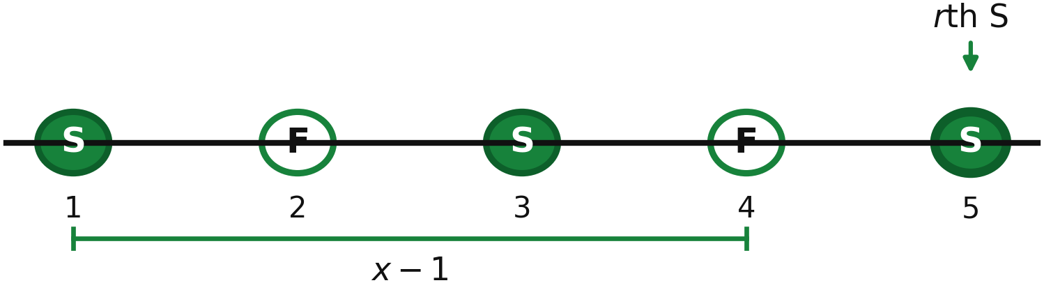
The number of ways to choose the locations of the first \(r-1\) successes among the first \(x-1\) trials is

\[\binom{x-1}{r-1}.\]

Every valid sequence contains exactly \(r\) successes and \(x-r\) failures. Therefore, the probability of any one valid sequence is

\[p^r q^{x-r}.\]

Multiplying the number of valid arrangements by the probability of one arrangement gives

Note

Negative Binomial PMF: total-trials convention

\[\boxed{ P(X=x) = \binom{x-1}{r-1}p^r(1-p)^{x-r} }\]

for

\[x=r,r+1,r+2,\ldots.\]

The combination is \(\binom{x-1}{r-1}\), not \(\binom{x}{r}\), because the last trial has already been fixed as a success.

3.5.6 Main Example: Third Success on Trial 5

Suppose independent trials have

\[p=0.40, \qquad q=0.60.\]

Let \(X\) be the total number of trials required to obtain the third success. Then

\[r=3.\]

Find the probability that the third success occurs on trial 5.

For \(X=5\), the fifth trial must be a success. Among the first four trials, exactly two must be successes. Therefore,

\[\binom{4}{2}=6\]

valid arrangements are possible.

For any one arrangement, there are three successes and two failures, so

\[P(\text{one valid arrangement}) = (0.40)^3(0.60)^2.\]

Hence,

\[P(X=5) = \binom42(0.40)^3(0.60)^2\]

\[= 6(0.064)(0.36) = 0.13824.\]

Thus, the probability that the third success occurs exactly on trial 5 is about \(13.8\%\).

3.5.7 Geometric Distribution as a Special Case

Set

\[r=1.\]

Then the negative binomial PMF becomes

\[P(X=x) = \binom{x-1}{0}p(1-p)^{x-1}.\]

Because

\[\binom{x-1}{0}=1,\]

we obtain

\[P(X=x) = (1-p)^{x-1}p, \qquad x=1,2,\ldots.\]

This is the geometric PMF. Therefore,

Note

The geometric distribution is the negative binomial distribution with \(r=1\).

3.5.8 Deriving the Mean and Variance

The mean and variance have a useful interpretation through geometric waiting times.

Let \(G_1\) be the number of trials required to obtain the first success, \(G_2\) the number of additional trials from the first success to the second success, and so on.

For \(r=3\), the waiting process can be viewed as three geometric blocks.

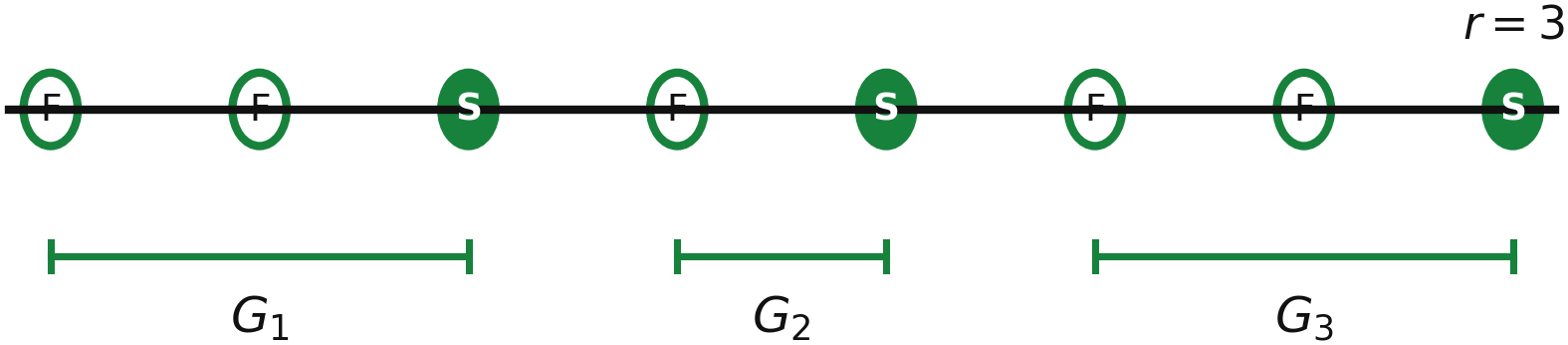
In general,

\[X=G_1+G_2+\cdots+G_r.\]

Each \(G_i\) is geometric with success probability \(p\), so

\[E(G_i)=\frac1p\]

and

\[\operatorname{Var}(G_i) = \frac{1-p}{p^2}.\]

Using linearity of expectation,

\[E(X) = E(G_1+G_2+\cdots+G_r)\]

\[= E(G_1)+E(G_2)+\cdots+E(G_r)\]

\[= r\left(\frac1p\right).\]

Therefore,

Note

Mean

\[\boxed{E(X)=\frac{r}{p}}.\]

For the variance, the waiting blocks are independent because the Bernoulli trials are independent. Therefore,

\[\operatorname{Var}(X) = \operatorname{Var}(G_1+\cdots+G_r)\]

\[= \operatorname{Var}(G_1)+\cdots+\operatorname{Var}(G_r)\]

\[= r\left(\frac{1-p}{p^2}\right).\]

Thus,

Note

Variance and Standard Deviation

\[\boxed{ \operatorname{Var}(X) = \frac{r(1-p)}{p^2} }\]

and

\[\boxed{ \sigma = \frac{\sqrt{r(1-p)}}{p} }.\]

3.5.9 Mean and Variance in the Main Example

For \(r=3\) and \(p=0.40\),

\[E(X) = \frac{3}{0.40} = 7.5.\]

The long-run average number of trials needed to obtain three successes is 7.5 trials.

The variance is

\[\operatorname{Var}(X) = \frac{3(0.60)}{(0.40)^2}\]

\[= \frac{1.8}{0.16} = 11.25.\]

The standard deviation is

\[\sigma = \sqrt{11.25} \approx 3.35.\]

The PMF is right-skewed because long waiting times are possible, although their probabilities become progressively smaller.

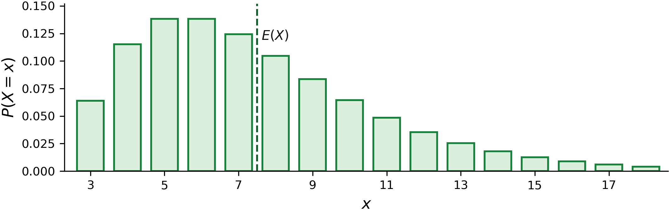
The expected value is not the most likely value and does not need to be an integer. It represents a long-run average waiting time.

3.5.10 Cumulative Probabilities and the Binomial Connection

The negative binomial distribution has a direct connection to the binomial distribution.

The event

\[X\leq x\]

means that the \(r\)-th success has occurred by trial \(x\). Equivalently, there must be at least :math:`r` successes among the first :math:`x` trials.

If

\[B\sim\operatorname{Binomial}(x,p),\]

then

\[P(X\leq x) = P(B\geq r).\]

Using the complement rule,

Note

\[\boxed{ P(X\leq x) = 1- \sum_{k=0}^{r-1} \binom{x}{k}p^k(1-p)^{x-k} }.\]

Similarly,

\[P(X>x) = P(B\leq r-1).\]

For the main example, \(r=3\), \(p=0.40\), and \(x=5\):

\[P(X\leq5) = P(B\geq3), \qquad B\sim\operatorname{Binomial}(5,0.40).\]

Therefore,

\[P(X\leq5) = 1- \left[P(B=0)+P(B=1)+P(B=2)\right]\]

\[= 0.31744.\]

Notice that \(P(X=5)=0.13824\) and \(P(X\leq5)=0.31744\) answer different questions. The first asks for the third success exactly on trial 5, whereas the second asks whether the third success has occurred by trial 5.

3.5.11 Failure-Count Form of the Negative Binomial

Some references define

\[Y=X-r\]

as the number of failures before the \(r\)-th success. If \(Y=y\), then the total number of trials is

\[X=y+r.\]

Substituting \(x=y+r\) into the total-trials PMF gives

\[P(Y=y) = \binom{y+r-1}{r-1}p^r(1-p)^y,\]

for

\[y=0,1,2,\ldots.\]

Because \(Y=X-r\), subtracting the constant \(r\) changes the mean but not the variance:

\[E(Y) = E(X)-r = \frac{r}{p}-r = \frac{r(1-p)}{p},\]

while

\[\operatorname{Var}(Y) = \operatorname{Var}(X) = \frac{r(1-p)}{p^2}.\]

This convention difference is one of the most common sources of conflicting negative binomial formulas.

3.5.12 Binomial Versus Negative Binomial

The two models use the same Bernoulli-trial assumptions, but they stop the experiment differently.

Feature	Binomial	Negative binomial
Fixed quantity	Trials \(n\)	Required successes \(r\)
Random quantity	Number of successes	Number of trials
Random variable	\(X=\text{successes in }n\text{ trials}\)	\(X=\text{trials until }r\text{-th success}\)
Support	\(0,1,\ldots,n\)	\(r,r+1,\ldots\)
Typical question	How many successes occur?	How long until enough successes occur?

A useful diagnostic question is:

What is fixed: the number of trials or the number of successes?

3.5.13 Effect of the Parameters

For a fixed \(r\), increasing \(p\) makes successes occur more often. The distribution therefore shifts toward smaller values of \(X\), and both the mean and variance decrease.

For a fixed \(p\), increasing \(r\) increases the required number of successes. The expected number of trials therefore increases because

\[E(X)=\frac{r}{p}.\]

The variance also increases linearly with \(r\):

\[\operatorname{Var}(X) = \frac{r(1-p)}{p^2}.\]

3.5.14 A Simple Method

For a negative binomial problem:

1. Define what counts as a success.

2. Identify the success probability \(p\).

3. Check independence and constant \(p\).

4. Identify the required number of successes \(r\).

5. Define whether the random variable counts total trials or failures.

6. For an exact total-trials probability, use

   \[P(X=x) = \binom{x-1}{r-1}p^r(1-p)^{x-r}.\]

7. For a by trial x question, translate the problem to a binomial cumulative probability if convenient.

8. Interpret the answer in terms of waiting for the required success.

3.5.15 Quick Practice

A basketball player makes each free throw with probability

\[p=0.75.\]

Assume attempts are independent. Let \(X\) be the number of attempts required to make the second basket.

Find:

1. \(P(X=3)\);

2. \(E(X)\);

3. \(\operatorname{Var}(X)\).

Answer

Here,

\[r=2, \qquad p=0.75, \qquad q=0.25.\]

For the second success to occur on attempt 3, exactly one success must occur among the first two attempts and the third attempt must be a success:

\[P(X=3) = \binom21(0.75)^2(0.25) = 0.28125.\]

The mean is

\[E(X) = \frac{2}{0.75} \approx 2.67.\]

The variance is

\[\operatorname{Var}(X) = \frac{2(0.25)}{(0.75)^2} \approx 0.889.\]

3.5.16 Common Mistakes

Do not confuse negative binomial with binomial. In a binomial model, the number of trials is fixed. In a negative binomial model, the required number of successes is fixed.

Do not use

\[\binom{x}{r}\]

for the total-trials PMF. If the \(r\)-th success occurs on trial \(x\), the final trial is already fixed as a success, leaving only \(x-1\) positions for the first \(r-1\) successes.

Do not allow \(x<r\). This is impossible when \(X\) counts total trials.

Do not confuse exactly on trial x with by trial x. They correspond to \(P(X=x)\) and \(P(X\leq x)\), respectively.

Do not mix the total-trials and failure-count conventions. Always define the random variable first.

3.5.17 Summary

For independent Bernoulli trials with constant success probability \(p\), let \(X\) be the number of trials required to obtain the \(r\)-th success.

Then

\[X=r,r+1,r+2,\ldots\]

and

\[\boxed{ P(X=x) = \binom{x-1}{r-1}p^r(1-p)^{x-r} }.\]

The geometric distribution is the special case \(r=1\).

The mean is

\[\boxed{E(X)=\frac rp},\]

and the variance is

\[\boxed{ \operatorname{Var}(X) = \frac{r(1-p)}{p^2} }.\]

For cumulative probabilities,

\[P(X\leq x) = P\bigl(\operatorname{Binomial}(x,p)\geq r\bigr).\]

The central modeling distinction is:

Binomial: fix trials and count successes.

Negative binomial: fix successes and count trials.