3.3 Binomial Distribution

Key Terms

Bernoulli trial（伯努利試驗）

A random experiment with exactly two possible categories, usually called success and failure.

Bernoulli random variable（伯努利隨機變數）

A 0–1 random variable representing the result of one Bernoulli trial.

Binomial random variable（二項隨機變數）

The number of successes in a fixed number of independent Bernoulli trials.

Binomial coefficient（二項係數）

The number \(\binom{n}{x}\) of ways to choose \(x\) success positions among \(n\) trials.

Success probability（成功機率）

The probability \(p\) of the category being counted on each trial.

Failure probability（失敗機率）

The probability \(q=1-p\) of the other category on each trial.

3.3.1 Learning Outcomes

After completing this section, students should be able to:

• explain what a Bernoulli trial is;

• define a Bernoulli random variable and write its PMF;

• derive the mean and variance of a Bernoulli random variable;

• determine whether a repeated-trial experiment satisfies the binomial conditions;

• explain how repeated Bernoulli trials produce a binomial random variable;

• recognize a Bernoulli random variable as the special case \(n=1\) of a binomial random variable;

• derive the binomial PMF from one success pattern and the number of possible arrangements;

• calculate exact binomial probabilities;

• use cumulative probabilities and complements for events such as at least and at most;

• derive the binomial mean and variance from Bernoulli indicator variables;

• interpret the effect of \(n\) and \(p\) on the shape of a binomial distribution.

3.3.2 From Uniform to Binomial

The discrete uniform distribution assigns the same probability to every possible value.

Many repeated-trial problems do not have this property. For example, suppose a student guesses on 10 multiple-choice questions with four choices per question. If

\[X=\text{number of correct answers},\]

then

\[X\in\{0,1,\ldots,10\},\]

but these 11 values are not equally likely.

The experiment consists instead of repeated correct/incorrect trials with a fixed success probability. This leads to the Bernoulli and binomial models.

3.3.3 Bernoulli Trials

The basic building block of a binomial experiment is a Bernoulli trial.

A Bernoulli trial has exactly two possible categories. Examples include:

• defective / non-defective;

• correct / incorrect;

• pass / fail;

• arrival / no arrival;

• error / correct transmission.

We call the category being counted success, even when it is not desirable. For example, defective may be defined as success when \(X\) counts number of defectives.

Let

\[p=P(\text{success})\]

and define

\[q=P(\text{failure})=1-p.\]

Thus,

\[p+q=1.\]

The two possible results of one Bernoulli trial are illustrated below.

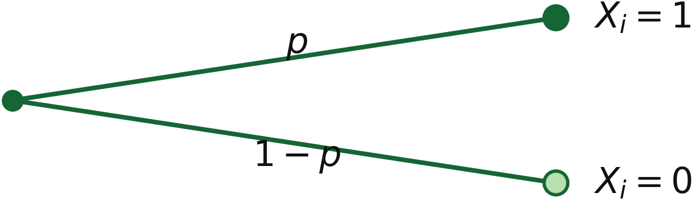
The probability \(p\) does not have to be larger than \(q\). It simply identifies the probability of the category called success.

3.3.4 The Bernoulli Random Variable

A Bernoulli trial can be represented numerically by a 0–1 random variable. Let

\[\begin{split}X= \begin{cases} 1, & \text{if success occurs},\\ 0, & \text{if failure occurs}. \end{cases}\end{split}\]

Then

\[X\sim\operatorname{Bernoulli}(p).\]

Its PMF is

\[P(X=x) = p^x(1-p)^{1-x}, \qquad x\in\{0,1\}.\]

This compact formula gives

\[P(X=1)=p\]

and

\[P(X=0)=1-p.\]

A Bernoulli random variable is also the special binomial case

\[X\sim\operatorname{Binomial}(1,p).\]

This gives a direct bridge from one Bernoulli trial to repeated Bernoulli trials.

3.3.5 Mean and Variance of a Bernoulli Random Variable

Because \(X\) takes only the values 0 and 1, its mean can be derived directly:

\[E(X) = 0(1-p)+1(p) = p.\]

Thus,

\[\boxed{E(X)=p}.\]

For the variance, first compute

\[E(X^2) = 0^2(1-p)+1^2(p) = p.\]

Using

\[\operatorname{Var}(X) = E(X^2)-[E(X)]^2,\]

we obtain

\[\operatorname{Var}(X) = p-p^2 = p(1-p).\]

Therefore,

\[\boxed{\operatorname{Var}(X)=p(1-p)}.\]

For one Bernoulli trial, the expected value equals the probability of success. The variance is largest at \(p=0.5\) and becomes small when \(p\) is close to 0 or 1.

3.3.6 From Bernoulli to Binomial

Now repeat the same type of Bernoulli trial \(n\) times.

Let

\[\begin{split}X_i= \begin{cases} 1, & \text{if trial }i\text{ is a success},\\ 0, & \text{otherwise}. \end{cases}\end{split}\]

The total number of successes is

\[X=X_1+X_2+\cdots+X_n.\]

If the Bernoulli trials are independent and all use the same success probability \(p\), then

\[X\sim\operatorname{Binomial}(n,p).\]

A shorter notation sometimes used is

\[X\sim B(n,p).\]

The two parameters are \(n\), the number of trials, and \(p\), the success probability on each trial.

The possible values are

\[X\in\{0,1,2,\ldots,n\}.\]

A Bernoulli random variable therefore describes one trial, while a binomial random variable counts successes across repeated Bernoulli trials.

3.3.7 Conditions for a Binomial Experiment

A binomial model requires four conditions.

Note

Binomial Conditions

1. The number of trials \(n\) is fixed.

2. Each trial has two possible categories.

3. The trials are independent.

4. The success probability \(p\) is constant from trial to trial.

The word independent is essential. Knowing the result of one trial should not change the probability model for another trial.

The trials should also be carried out under the same probability conditions, so the same \(p\) applies on every trial. In this sense, the repeated Bernoulli trials are identically modeled even though their observed outcomes may differ.

For example, 20 customers independently choosing between self-checkout and a counter can be modeled as binomial if each customer has the same probability of choosing self-checkout.

In contrast, repeatedly drawing cards without replacement generally does not satisfy the binomial conditions because the composition of the deck changes after each draw.

3.3.8 Deriving the Binomial PMF

Suppose \(X=x\), meaning that exactly \(x\) successes occur in \(n\) trials.

Consider one particular arrangement containing \(x\) successes and \(n-x\) failures. Because the trials are independent, the probability of that specific arrangement is

\[p^x(1-p)^{n-x}.\]

However, the \(x\) successes can occur in different positions. The number of ways to choose the success positions is

\[\binom{n}{x} = \frac{n!}{x!(n-x)!}.\]

Therefore,

Note

Binomial Probability Mass Function

If

\[X\sim\operatorname{Binomial}(n,p),\]

then

\[\boxed{ P(X=x) = \binom{n}{x}p^x(1-p)^{n-x} }\]

for

\[x=0,1,\ldots,n.\]

The formula can be read as

\[\underbrace{\binom{n}{x}}_{\text{number of arrangements}} \times \underbrace{p^x(1-p)^{n-x}}_{\text{probability of one arrangement}}.\]

3.3.9 Why the Binomial Coefficient Appears

Consider \(n=4\) trials and suppose exactly two successes occur.

The two successes can occupy six different pairs of positions. The figure below shows all six arrangements using dark blocks for success and light blocks for failure.

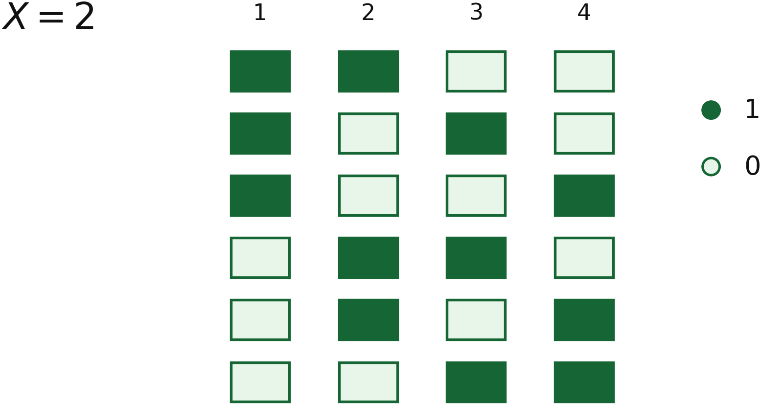
The number of arrangements is

\[\binom42=6.\]

Every arrangement has the same probability

\[p^2(1-p)^2.\]

Adding the six mutually exclusive arrangements gives

\[P(X=2) = \binom42p^2(1-p)^2.\]

This is the combinatorial reasoning behind the binomial coefficient.

3.3.10 Example 1: Bit Errors in Digital Communication

A digital communication channel has bit error probability

\[p=0.10.\]

Assume bit errors occur independently. Four bits are transmitted, and let

\[X=\text{number of error bits among the four transmitted bits}.\]

Then

\[X\sim\operatorname{Binomial}(4,0.10).\]

Find the probability of exactly two errors.

A particular pattern containing two errors and two correct bits has probability

\[(0.10)^2(0.90)^2 = 0.0081.\]

There are

\[\binom42=6\]

ways to choose the two error positions. Therefore,

\[P(X=2) = \binom42(0.10)^2(0.90)^2 = 6(0.0081) = 0.0486.\]

Thus, about \(4.86\%\) of such four-bit transmissions contain exactly two errors under this model.

3.3.11 Binomial CDF and Probability Language

The binomial PMF gives probabilities for exact values. For cumulative events, we add PMF values.

For

\[X\sim\operatorname{Binomial}(n,p),\]

at most \(x\) successes means

\[P(X\le x) = \sum_{k=0}^{x} \binom nk p^k(1-p)^{n-k}.\]

This is the binomial CDF:

\[F(x)=P(X\le x).\]

Common translations include:

Words	Probability notation
exactly \(x\)	\(P(X=x)\)
at most \(x\)	\(P(X\le x)\)
fewer than \(x\)	\(P(X<x)\)
at least \(x\)	\(P(X\ge x)\)
more than \(x\)	\(P(X>x)\)

Complements are often useful. For example,

\[P(X\ge1) = 1-P(X=0) = 1-(1-p)^n.\]

Similarly,

\[P(X>k) = 1-P(X\le k).\]

3.3.12 Deriving the Mean and Variance of a Binomial Distribution

Let

\[X=X_1+X_2+\cdots+X_n,\]

where the \(X_i\) are independent Bernoulli random variables with

\[E(X_i)=p\]

and

\[\operatorname{Var}(X_i)=p(1-p).\]

Using linearity of expectation,

\[E(X) = E(X_1+\cdots+X_n) = E(X_1)+\cdots+E(X_n).\]

Therefore,

\[E(X) = p+p+\cdots+p = np.\]

Thus,

\[\boxed{E(X)=np}.\]

For the variance,

\[\operatorname{Var}(X) = \operatorname{Var}(X_1+\cdots+X_n).\]

Because the Bernoulli trials are independent, their variances add:

\[\operatorname{Var}(X) = \operatorname{Var}(X_1)+\cdots+\operatorname{Var}(X_n).\]

Hence,

\[\operatorname{Var}(X) = p(1-p)+\cdots+p(1-p) = np(1-p).\]

Therefore, writing \(q=1-p\),

\[\boxed{\operatorname{Var}(X)=np(1-p)=npq}\]

and

\[\boxed{\sigma=\sqrt{np(1-p)}}.\]

The independence condition is what allows the variances of the individual Bernoulli trials to be added directly.

3.3.13 Example 2: Quality Control

A manufacturing machine produces an item with defect probability

\[p=0.03.\]

Suppose 200 independently produced items are inspected. Let

\[X=\text{number of defective items among the 200 inspected items}.\]

Then

\[X\sim\operatorname{Binomial}(200,0.03).\]

The mean is

\[E(X) = np = 200(0.03) = 6.\]

The variance is

\[\operatorname{Var}(X) = np(1-p) = 200(0.03)(0.97) = 5.82.\]

The standard deviation is

\[\sigma = \sqrt{5.82} \approx 2.41.\]

Thus, the long-run average is about 6 defectives per group of 200, while the actual count naturally fluctuates around this value.

3.3.14 Shape of a Binomial Distribution

The shape of a binomial PMF depends on both \(n\) and \(p\).

For a fixed \(n\):

• when \(p=0.5\), the distribution is symmetric;

• when \(p<0.5\), probability is concentrated toward smaller counts and the distribution is typically right-skewed;

• when \(p>0.5\), probability is concentrated toward larger counts and the distribution is typically left-skewed.

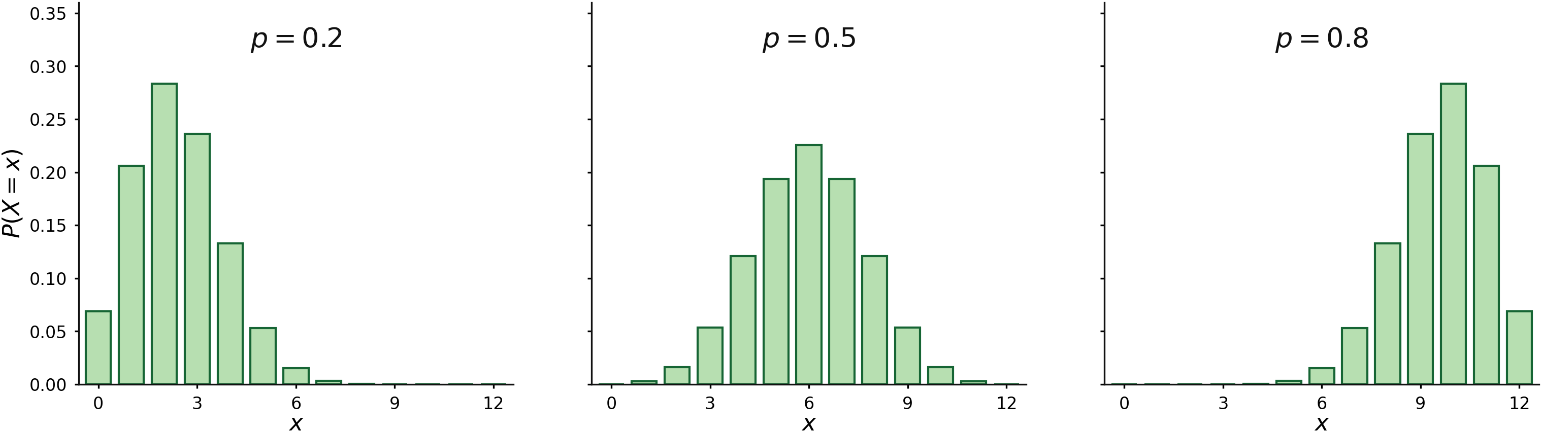
As \(n\) increases, the number of possible success counts increases and the PMF often appears smoother. Probability tends to concentrate around the mean

\[np.\]

The parameters therefore have different roles: \(p\) strongly controls where the distribution is concentrated and its skew direction, while \(n\) affects the number of possible counts and the overall scale of the distribution.

3.3.15 Additional: The Most Likely Number of Successes

The mode is the value of \(x\) for which \(P(X=x)\) is largest. One way to locate it is to compare neighboring PMF values:

\[\frac{P(X=x+1)}{P(X=x)} = \frac{n-x}{x+1} \frac{p}{1-p}.\]

If this ratio is greater than 1, the PMF is still increasing. If it is less than 1, the PMF is decreasing.

Let

\[m=(n+1)p.\]

If \(m\) is not an integer, the unique mode is

\[\lfloor m\rfloor.\]

If \(m\) is an integer, there are two adjacent modes:

\[m-1 \qquad\text{and}\qquad m.\]

For introductory calculations, directly comparing PMF values is also valid.

3.3.16 When the Binomial Model Does Not Apply

The binomial formula should not be used merely because a problem contains two categories.

For example, suppose items are sampled from a small finite batch without replacement. After each selection, the population composition changes. Therefore:

• the trials are not independent;

• the success probability changes from one draw to the next.

This is generally not a binomial experiment. Sampling without replacement from a finite population leads naturally to the hypergeometric distribution, which is considered separately.

3.3.17 A Simple Method

For a possible binomial problem:

1. Define what counts as success.

2. Identify the fixed number of trials \(n\).

3. Identify the success probability \(p\).

4. Check that each trial has two categories.

5. Check independence.

6. Check that \(p\) remains constant.

7. Define \(X\) as the number of successes.

8. Translate the requested event into notation.

9. Apply the PMF, CDF, or complement rule as appropriate.

A useful notation summary is

\[X\sim B(n,p),\qquad q=1-p.\]

For \(n=1\), this reduces to a Bernoulli random variable.

3.3.18 Common Mistakes

Do not use the binomial model without checking independence and constant \(p\).

Do not confuse \(n\), the total number of trials, with \(x\), the number of successes of interest.

Do not forget the combination factor \(\binom nx\) when calculating an exact binomial probability.

Do not interpret success as necessarily desirable. It simply identifies the category being counted.

Do not confuse a Bernoulli random variable with a binomial random variable: a Bernoulli random variable describes one 0–1 trial, while a binomial random variable counts successes across \(n\) trials.

3.3.19 Summary

A Bernoulli random variable has

\[P(X=1)=p, \qquad P(X=0)=1-p,\]

with

\[E(X)=p\]

and

\[\operatorname{Var}(X)=p(1-p).\]

A binomial random variable is the sum of \(n\) independent Bernoulli random variables with the same success probability:

\[X=X_1+\cdots+X_n \sim \operatorname{Binomial}(n,p).\]

Its PMF is

\[P(X=x) = \binom nx p^x(1-p)^{n-x}.\]

Its mean, variance, and standard deviation are

\[E(X)=np,\]

\[\operatorname{Var}(X)=np(1-p),\]

and

\[\sigma=\sqrt{np(1-p)}.\]

The central modeling question is not merely whether there are two outcomes. The experiment must satisfy the full repeated-Bernoulli structure: fixed \(n\), two categories, independence, and constant \(p\).