4.5 Normal Distribution

Key Terms

Normal distribution, mean, standard deviation, variance, standardization, z-score, percentile, critical value, continuity correction, normal approximation.

Learning Outcomes

After studying this section, you should be able to:

• describe the role of \(\mu\) and \(\sigma\) in a normal distribution;

• convert values on an original measurement scale to the standard-normal scale;

• calculate left-tail, right-tail, and interval probabilities;

• find percentiles and cutoff values from probabilities;

• interpret probabilities as areas under a normal density;

• use a normal distribution to approximate selected discrete distributions;

• apply the \(0.5\) continuity correction correctly.

4.5.1 From the Standard Normal to the Normal Family

Section 4.4 introduced the standard normal random variable

\[Z\sim N(0,1).\]

The standard normal distribution is one member of a much larger family. A general normal random variable may have any real-valued center and any positive standard deviation.

Normal models often appear when an observed quantity is affected by many small influences. Examples include measurement error, process dimensions, biological measurements, test scores, and aggregated random effects.

The key idea for probability calculations is simple:

Every normal distribution can be converted to the same standard-normal reference scale.

Thus, the \(z\)-skills from Section 4.4 are the computational tool for working with all normal distributions.

4.5.2 Definition and Parameters

A continuous random variable \(X\) follows a normal distribution if its density has the form

\[f(x) = \frac{1}{\sigma\sqrt{2\pi}} \exp\left[ -\frac{(x-\mu)^2}{2\sigma^2} \right], \qquad -\infty<x<\infty,\]

where

\[-\infty<\mu<\infty, \qquad \sigma>0.\]

In this handout, the notation is

\[X\sim N(\mu,\sigma^2),\]

so the second argument is the variance.

The parameters have distinct roles:

• \(\mu\) controls location;

• \(\sigma\) controls spread;

• \(\sigma^2\) is the variance.

For a normal random variable,

\[E(X)=\mu, \qquad \operatorname{Var}(X)=\sigma^2.\]

The density is symmetric around \(\mu\), and the mean, median, and mode coincide at the center.

Changing \(\mu\) shifts the curve. Changing \(\sigma\) changes the width and height while the total area remains 1.

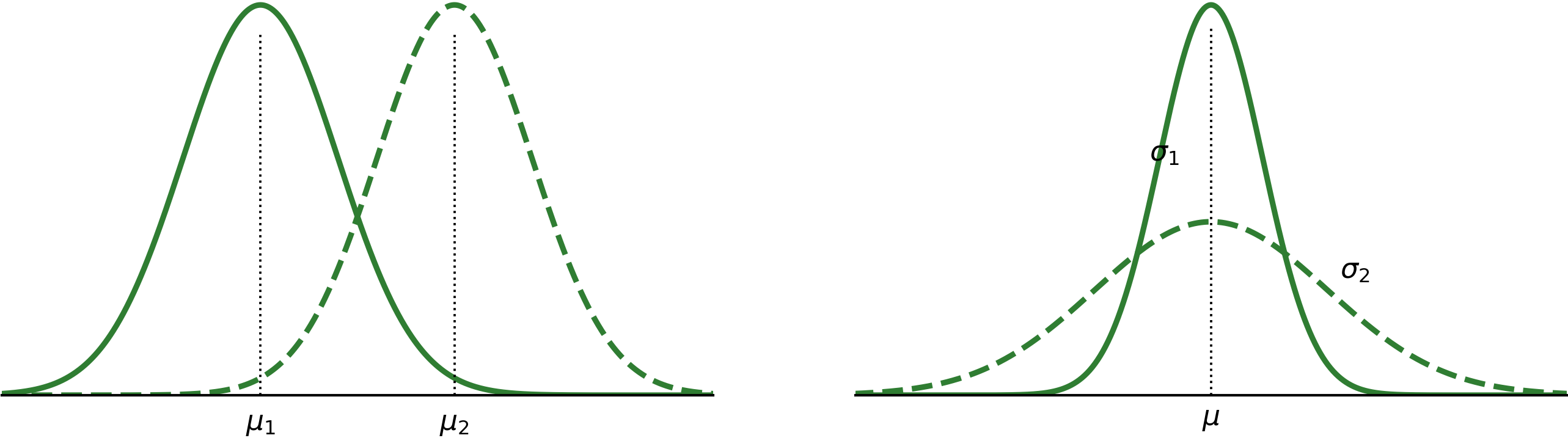
The left plot illustrates a location change. The right plot keeps the center fixed and changes the spread. A larger \(\sigma\) produces a wider, lower curve because the total probability area must remain equal to 1.

4.5.3 Probabilities Are Areas

For any continuous random variable,

\[P(X=x)=0.\]

Therefore,

\[P(X<x)=P(X\leq x)\]

and

\[P(X>x)=P(X\geq x).\]

For a normal random variable, probabilities are areas under the density curve. The general normal CDF does not have a simple elementary formula. Instead, we standardize the relevant boundary and use the standard normal CDF

\[\Phi(z)=P(Z\leq z).\]

4.5.4 Standardization: Moving from X to Z

Suppose

\[X\sim N(\mu,\sigma^2).\]

Then

Note

Standardization

\[Z = \frac{X-\mu}{\sigma} \sim N(0,1).\]

For a particular value \(x\),

\[z=\frac{x-\mu}{\sigma}.\]

The transformation subtracts the location and divides by the scale. Probability is preserved under this one-to-one transformation.

For example, suppose electrical current is modeled as

\[X\sim N(10,2^2).\]

Then \(x=13\) corresponds to

\[z = \frac{13-10}{2} = 1.5.\]

Therefore,

\[P(X>13) = P(Z>1.5).\]

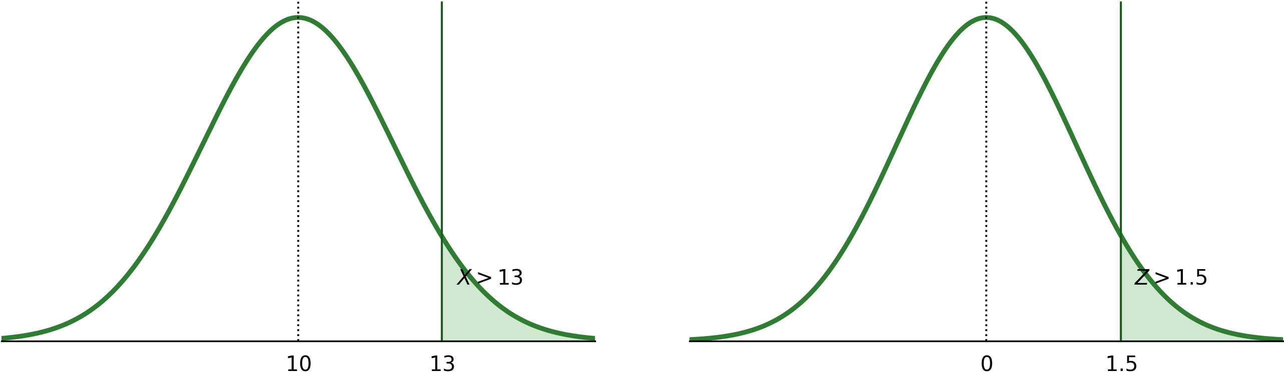
The numerical scale changes, but the shaded probability area does not.

The reverse transformation is equally important:

\[x=\mu+z\sigma.\]

This form is used when a probability or percentile is given and the original measurement value is unknown.

4.5.5 Three Basic Probability Patterns

Let

\[z_x=\frac{x-\mu}{\sigma}.\]

For a left-tail probability,

\[P(X<x) = \Phi(z_x).\]

For a right-tail probability,

\[P(X>x) = 1-\Phi(z_x).\]

For an interval \(a<X<b\),

\[P(a<X<b) = \Phi\left(\frac{b-\mu}{\sigma}\right) - \Phi\left(\frac{a-\mu}{\sigma}\right).\]

These formulas are simply the probability patterns from Section 4.4 written on an arbitrary normal measurement scale.

4.5.6 Example: Electrical Current

Suppose an industrial engineer models current in a wire as

\[X\sim N(10,2^2),\]

where current is measured in milliamperes.

(a) Probability that current exceeds 13 mA

Standardize:

\[z=\frac{13-10}{2}=1.50.\]

Then

\[P(X>13) = P(Z>1.50) = 1-\Phi(1.50).\]

Using

\[\Phi(1.50)\approx0.9332,\]

we obtain

\[P(X>13) \approx 1-0.9332 = 0.0668.\]

So a current above 13 mA is unusual, but not impossible.

(b) Probability that current is below 13.06 mA

\[z = \frac{13.06-10}{2} = 1.53.\]

Therefore,

\[P(X<13.06) = \Phi(1.53) \approx 0.9370.\]

(c) Probability that current lies between 7.50 and 10.74 mA

The two standardized boundaries are

\[z_1 = \frac{7.50-10}{2} = -1.25\]

and

\[z_2 = \frac{10.74-10}{2} = 0.37.\]

Hence,

\[P(7.50<X<10.74) = \Phi(0.37)-\Phi(-1.25) \approx 0.6443-0.1056 = 0.5387.\]

4.5.7 Percentiles and Critical Values

Sometimes we know the probability and need the value on the original scale.

Suppose

\[P(X<k)=r.\]

First find \(z_r\) such that

\[\Phi(z_r)=r.\]

Then convert back to the original scale:

\[k=\mu+z_r\sigma.\]

The value \(k\) is the percentile corresponding to cumulative probability \(r\) (the \(100r\) percentile).

For example, exam scores have

\[X\sim N(63,5^2).\]

Find the 90th percentile. From the standard normal distribution,

\[z_{0.90}\approx1.2816.\]

Thus,

\[k = 63+1.2816(5) \approx 69.4.\]

So approximately 90% of scores lie below 69.4.

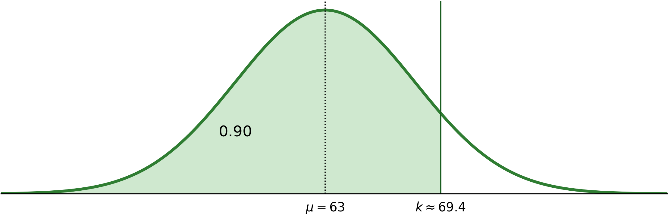
The same method works for quartiles, deciles, specification cutoffs, and other critical values.

4.5.8 Translating the 68–95–99.7 Rule Back to X

Section 4.4 established the standard-normal landmarks

\[P(-1<Z<1)\approx0.6827,\]

\[P(-2<Z<2)\approx0.9545,\]

and

\[P(-3<Z<3)\approx0.9973.\]

For a general normal random variable, these become

\[P(\mu-\sigma<X<\mu+\sigma)\approx0.6827,\]

\[P(\mu-2\sigma<X<\mu+2\sigma)\approx0.9545,\]

and

\[P(\mu-3\sigma<X<\mu+3\sigma)\approx0.9973.\]

These are useful for interpretation and as a quick reasonableness check. For precise probabilities, use standardization and \(\Phi\).

4.5.9 A Practical Workflow for Normal Problems

1. Identify the random variable and its units.

2. Write the model using \(X\sim N(\mu,\sigma^2)\).

3. Sketch or identify the required area: left, right, or between.

4. Standardize each boundary using

   \[z=\frac{x-\mu}{\sigma}.\]

5. Use the standard normal table or software to obtain \(\Phi(z)\).

6. Apply a complement or subtraction if needed.

7. Interpret the result in the original context.

For a percentile problem, reverse Steps 4–5:

\[r \longrightarrow z_r \longrightarrow x=\mu+z_r\sigma.\]

4.5.10 Why a Continuous Normal Curve Can Approximate Discrete Counts

A normal distribution is continuous, yet it can approximate several discrete count distributions when the discrete probability mass becomes sufficiently smooth and mound-shaped.

This is useful when an exact discrete probability would require many terms. The approximation also shows why the standardization idea is broader than the normal family itself.

The main cases in this course are:

• binomial counts;

• Poisson counts;

• hypergeometric counts under suitable conditions.

The important extra step is the continuity correction.

4.5.11 Continuity Correction

A discrete value \(X=k\) represents an entire bar centered at the integer \(k\). A continuous normal curve represents that bar by the interval

\[k-0.5<Y<k+0.5.\]

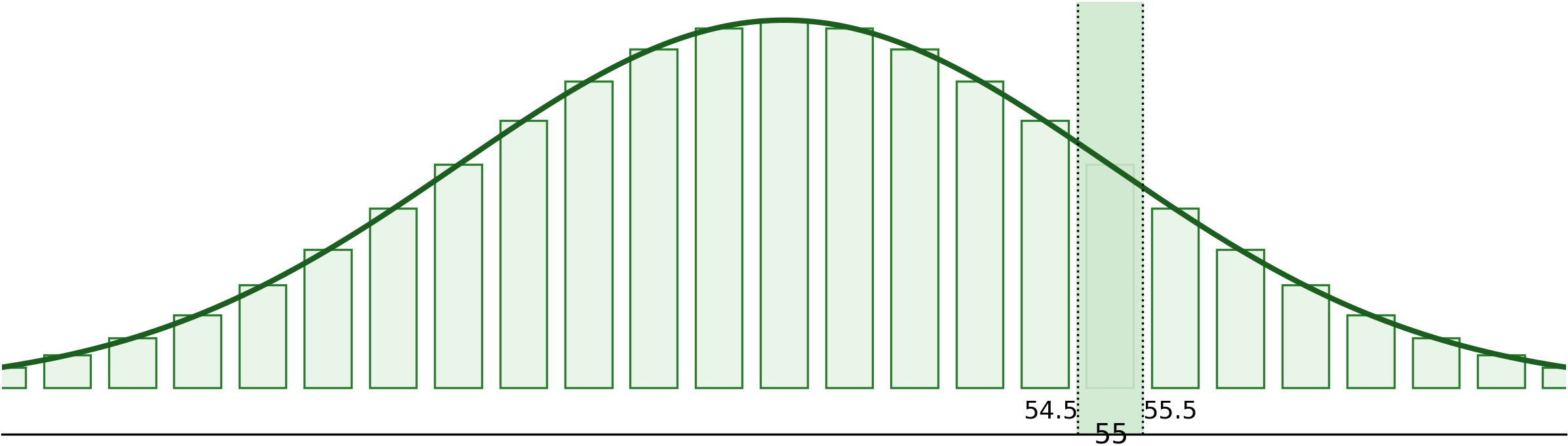
This leads to the following useful translations.

Discrete event	Continuous approximation
\(P(X\leq k)\)	\(P(Y<k+0.5)\)
\(P(X<k)\)	\(P(Y<k-0.5)\)
\(P(X\geq k)\)	\(P(Y>k-0.5)\)
\(P(X>k)\)	\(P(Y>k+0.5)\)
\(P(X=k)\)	\(P(k-0.5<Y<k+0.5)\)
\(P(a\leq X\leq b)\)	\(P(a-0.5<Y<b+0.5)\)

The correction is applied before standardization.

4.5.12 Normal Approximation to the Binomial

Suppose

\[X\sim\operatorname{Binomial}(n,p).\]

Then

\[\mu=np, \qquad \sigma^2=np(1-p).\]

When the binomial distribution is not strongly skewed, use

\[Y\sim N\left(np,\,np(1-p)\right).\]

A common introductory check is

\[np\geq5 \qquad\text{and}\qquad n(1-p)\geq5.\]

If either quantity is small, the binomial distribution may be too skewed for a good symmetric normal approximation.

Example

Let

\[X\sim\operatorname{Binomial}(100,0.50).\]

Approximate

\[P(X\leq55).\]

The normal approximation has

\[\mu=100(0.50)=50\]

and

\[\sigma = \sqrt{100(0.50)(0.50)} =5.\]

Apply the continuity correction:

\[P(X\leq55) \approx P(Y<55.5).\]

Standardize:

\[z = \frac{55.5-50}{5} = 1.10.\]

Therefore,

\[P(X\leq55) \approx \Phi(1.10) \approx 0.8643.\]

The exact binomial probability is approximately

\[0.8644,\]

so the approximation is very close in this case.

Without the continuity correction, using \(55\) instead of \(55.5\) would give \(\Phi(1)=0.8413\), which is noticeably less accurate.

4.5.13 When Is the Binomial Approximation Good?

The quality depends strongly on the shape of the original discrete distribution.

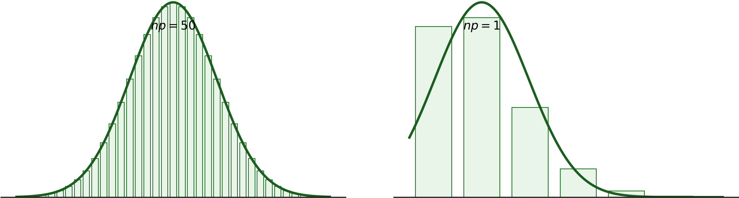
When both \(np\) and \(n(1-p)\) are reasonably large, the binomial mass is much more symmetric and the normal curve can track it well. If \(p\) is very close to 0 or 1 and the sample size is not large enough, the binomial mass remains strongly skewed.

4.5.14 Normal Approximation to the Poisson

Suppose

\[X\sim\operatorname{Poisson}(\lambda).\]

Because

\[E(X)=\lambda, \qquad \operatorname{Var}(X)=\lambda,\]

we use

\[Y\sim N(\lambda,\lambda).\]

Thus,

\[\sigma=\sqrt{\lambda}.\]

The same continuity correction is used.

Example

Suppose

\[X\sim\operatorname{Poisson}(20).\]

Approximate

\[P(X\leq15).\]

Use

\[Y\sim N(20,20).\]

The corrected cutoff is

\[15.5.\]

Therefore,

\[z = \frac{15.5-20}{\sqrt{20}} \approx -1.006.\]

Hence,

\[P(X\leq15) \approx \Phi(-1.006) \approx 0.1572.\]

The exact Poisson probability is approximately \(0.1565\).

As \(\lambda\) becomes larger, the Poisson distribution becomes less skewed and the normal approximation generally improves.

4.5.15 Normal Approximation to the Hypergeometric

Suppose a population has size \(N\), with \(K\) successes, and a sample of size \(n\) is selected without replacement. Let

\[p=\frac KN.\]

For a hypergeometric count \(X\),

\[\mu=np\]

and

\[\sigma^2 = np(1-p) \left(\frac{N-n}{N-1}\right).\]

When the count distribution is sufficiently smooth, approximate with

\[Y\sim N(\mu,\sigma^2)\]

and use the continuity correction.

Example

Suppose

\[N=100, \qquad K=20, \qquad n=10.\]

Then

\[p=0.20, \qquad \mu=10(0.20)=2,\]

and

\[\sigma^2 = 10(0.20)(0.80) \left(\frac{90}{99}\right) \approx1.4545.\]

To approximate \(P(X\leq3)\), use the corrected boundary \(3.5\):

\[z = \frac{3.5-2}{\sqrt{1.4545}} \approx1.244.\]

Therefore,

\[P(X\leq3) \approx \Phi(1.244) \approx0.8932.\]

The exact hypergeometric probability is approximately \(0.8904\).

When the sampling fraction \(n/N\) is very small, the finite population correction is close to 1, so the hypergeometric model is also close to a binomial model.

4.5.16 Choosing Between Exact and Approximate Methods

Use an exact discrete distribution when:

• the exact probability is easy to compute;

• the count distribution is strongly skewed;

• the approximation conditions are poor;

• high numerical accuracy is important.

A normal approximation is useful when:

• the discrete count is large enough to appear smooth;

• exact calculation is cumbersome;

• a quick approximation is sufficient;

• the continuity correction can be applied clearly.

An approximation should not be treated as an exact identity.

4.5.17 Practice Set

Normal probability calculations

1. Suppose \(X\sim N(70,10^2)\). Find \(P(X>82)\).

2. Suppose \(X\sim N(50,6^2)\). Find \(P(44<X<62)\).

3. Suppose \(X\sim N(100,15^2)\). Find \(P(X<85)\).

Percentiles and cutoffs

4. Exam scores follow \(N(63,5^2)\). Find the 90th percentile.

5. Daily computer-use time follows \(N(2,0.5^2)\). Find the 25th percentile.

6. Mandarin-orange diameters follow \(N(5.85,0.24^2)\). Find the symmetric interval containing the middle 80% of diameters.

Normal approximation to discrete distributions

7. Let \(X\sim\operatorname{Binomial}(100,0.50)\). Approximate \(P(X\leq55)\) using a continuity correction.

8. Let \(X\sim\operatorname{Binomial}(50,0.10)\). Approximate \(P(X=5)\) using a continuity correction.

9. Let \(X\sim\operatorname{Poisson}(20)\). Approximate \(P(X\geq25)\).

10. For a hypergeometric model with \(N=100\), \(K=20\), and \(n=10\), approximate \(P(X\leq3)\) using the normal model with finite population correction.

Concept checks

11. Why does \(P(X<65)=P(X\leq65)\) for a normal random variable?

12. Why is \(np=2\) a warning sign when using a normal approximation to a binomial distribution?

13. For a discrete probability \(P(X=12)\), what interval is used under a continuity-corrected normal approximation?

4.5.18 Practice Answers

1. \[z=\frac{82-70}{10}=1.20, \qquad P(X>82)\approx0.1151.\]
2. \[z_1=-1, \qquad z_2=2,\]

   so

   \[P(44<X<62) = \Phi(2)-\Phi(-1) \approx0.8186.\]
3. \[z=-1, \qquad P(X<85)\approx0.1587.\]
4. \[63+1.2816(5)\approx69.4.\]
5. \[2+(-0.6745)(0.5)\approx1.663.\]

6. The middle 80% leaves 10% in each tail, so use \(z_{0.90}\approx1.2816\):

   \[5.85\pm1.2816(0.24) \approx (5.542,\,6.158).\]
7. \[P(X\leq55) \approx P(Y<55.5) \approx0.8643.\]

8. Here

   \[\mu=5, \qquad \sigma=\sqrt{4.5}\approx2.121.\]

   Use

   \[4.5<Y<5.5.\]

   Then

   \[P(X=5)\approx0.1863.\]

9. Use \(24.5\) as the corrected lower boundary:

   \[P(X\geq25) \approx P(Y>24.5) \approx0.1572.\]
10. \[P(X\leq3)\approx0.8932.\]

11. A single point has probability zero for a continuous random variable.

12. The binomial distribution is likely to remain strongly skewed because the expected number of successes is very small.

13. \[11.5<Y<12.5.\]

4.5.19 Common Mistakes

Using variance instead of standard deviation

The correct z-score is

\[z=\frac{x-\mu}{\sigma},\]

not \((x-\mu)/\sigma^2\).

Confusing the two normal-notation conventions

In this handout,

\[N(\mu,\sigma^2)\]

uses variance as the second parameter. Some software and textbooks instead list the standard deviation. Always check the convention being used.

Forgetting the direction of the probability

A cumulative table gives a left-tail probability. For a right tail, use a complement.

Applying the continuity correction after standardization

Correct the original discrete boundary first, then calculate the z-score.

Using a normal approximation for a strongly skewed count

Check the shape conditions before relying on the approximation.

Treating an approximation as exact

The normal approximation is a computational model. When feasible, an exact discrete probability remains the reference value.

4.5.20 Summary

A normal random variable is written in this handout as

\[X\sim N(\mu,\sigma^2).\]

Its mean and variance are

\[E(X)=\mu, \qquad \operatorname{Var}(X)=\sigma^2.\]

Every normal random variable can be standardized:

\[Z=\frac{X-\mu}{\sigma}.\]

Normal probabilities are therefore computed using the standard-normal CDF \(\Phi\).

For percentiles,

\[x=\mu+z\sigma.\]

The normal distribution can also approximate discrete count distributions. For the binomial,

\[\mu=np, \qquad \sigma=\sqrt{np(1-p)}.\]

For the Poisson,

\[\mu=\lambda, \qquad \sigma=\sqrt{\lambda}.\]

For the hypergeometric,

\[\mu=np, \qquad \sigma^2 = np(1-p)\frac{N-n}{N-1}.\]

Whenever a continuous normal curve approximates an integer-valued count, apply the appropriate \(0.5\) continuity correction.