4.4 Standard Normal Distribution and z-Scores

The purpose of this section is to build a standard reference scale for continuous probability calculations.

We will focus on the standard normal random variable \(Z\) and on using \(z\)-scores. The general normal distribution will be introduced in the next section.

Key Terms

• standard normal random variable

• z-score

• standardization

• cumulative probability

• left-tail probability

• right-tail probability

• standard normal table

• symmetry

4.4.1 Learning Objectives

After completing this section, you should be able to:

1. explain what a \(z\)-score represents;

2. compute a \(z\)-score from a value, mean, and standard deviation;

3. interpret positive, negative, and zero \(z\)-scores;

4. recognize the standard normal reference variable \(Z\);

5. use a cumulative standard normal table;

6. calculate left-tail, right-tail, and interval probabilities for \(Z\);

7. use symmetry and complements to simplify calculations;

8. find approximate \(z\)-values from cumulative probabilities.

4.4.2 The z-Score: A Standard Distance

Suppose a quantity has mean \(\mu\) and standard deviation \(\sigma\). For an observed value \(x\), define its z-score as

\[z=\frac{x-\mu}{\sigma}.\]

A \(z\)-score measures the distance from the mean in standard deviation units.

• \(z>0\): the value is above the mean;

• \(z<0\): the value is below the mean;

• \(z=0\): the value equals the mean;

• \(|z|\) tells how many standard deviations the value is from the mean.

For example, suppose a measurement has

\[\mu=10, \qquad \sigma=2.\]

If \(x=13\), then

\[z = \frac{13-10}{2} = 1.5.\]

Thus, 13 is 1.5 standard deviations above the mean.

If \(x=8\), then

\[z = \frac{8-10}{2} = -1.\]

Thus, 8 is 1 standard deviation below the mean.

Note

A \(z\)-score has no physical unit. The original unit cancels when dividing by the standard deviation.

The relationship can also be reversed. From

\[z=\frac{x-\mu}{\sigma},\]

we obtain

\[x=\mu+z\sigma.\]

This form will become useful when we later convert a standardized value back to an original measurement scale.

4.4.3 Standardization Does Not Automatically Mean Normality

The calculation

\[z=\frac{x-\mu}{\sigma}\]

can be used to describe the relative position of a value on many different measurement scales.

However, computing a \(z\)-score does not by itself imply that the underlying variable has a normal distribution.

In this section, we separately study a specific reference random variable, called the standard normal random variable.

The next section will explain when an original random variable can be connected to this standard normal reference curve for probability calculations.

4.4.4 The Standard Normal Random Variable

A standard normal random variable is denoted by

\[Z.\]

It has

\[E(Z)=0\]

and

\[\operatorname{SD}(Z)=1.\]

Equivalently,

\[\operatorname{Var}(Z)=1.\]

The usual notation is

\[Z\sim N(0,1).\]

For now, treat \(N(0,1)\) as the name of this standard reference distribution. We will develop the general normal family in the next section.

Its density is symmetric about zero. For reference, the density is

\[\phi(z) = \frac{1}{\sqrt{2\pi}} e^{-z^2/2}, \qquad -\infty<z<\infty.\]

We will not calculate probabilities by integrating this function by hand. Instead, we will use its cumulative probability function.

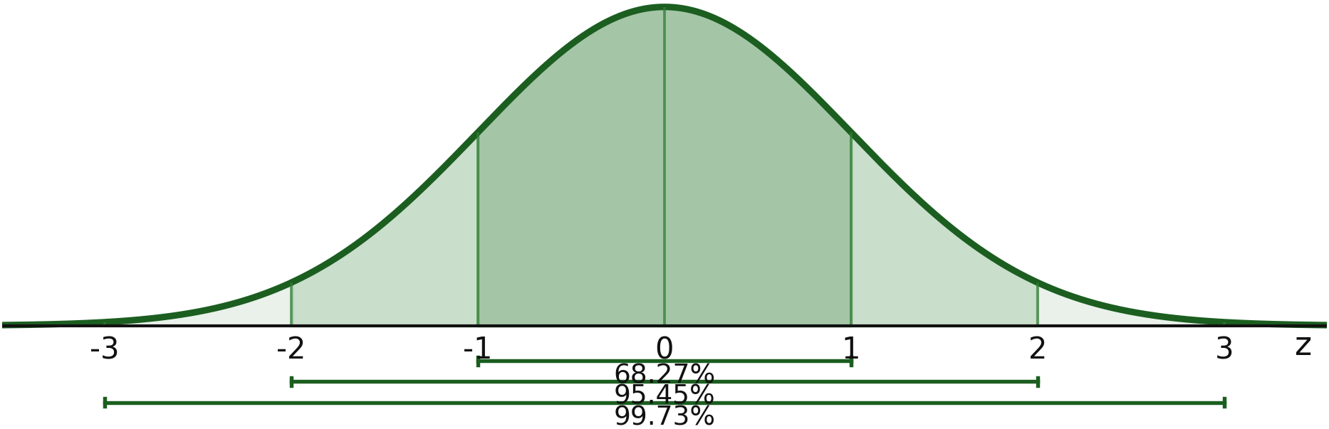
The horizontal scale is already measured in standard deviations. Therefore, \(z=1\) means one standard deviation above the mean and \(z=-2\) means two standard deviations below the mean.

Useful reference areas are

\[P(-1<Z<1)\approx0.6827,\]

\[P(-2<Z<2)\approx0.9545,\]

and

\[P(-3<Z<3)\approx0.9973.\]

These are useful landmarks for checking whether a probability calculation is reasonable.

4.4.5 The Standard Normal CDF

Define the cumulative distribution function

\[\Phi(z) = P(Z\leq z).\]

Because \(Z\) is continuous,

\[P(Z<z)=P(Z\leq z).\]

Thus,

\[\Phi(z)=P(Z<z).\]

Geometrically, \(\Phi(z)\) is the area under the standard normal curve to the left of \(z\).

The cumulative probability can also be written as

\[\Phi(z) = \int_{-\infty}^{z}\phi(t)\,dt.\]

This integral does not have a simple elementary antiderivative. Therefore, probabilities are normally obtained from a standard normal table or software.

4.4.6 Reading a Cumulative z-Table

This handout assumes a standard normal table whose entries are

\[\Phi(z)=P(Z<z).\]

Always check the heading of a table before using it because some tables use a different convention.

Suppose we want

\[P(Z<1.48).\]

To locate \(z=1.48\):

1. use \(1.4\) to locate the row;

2. use \(0.08\) to locate the column;

3. read the entry at their intersection.

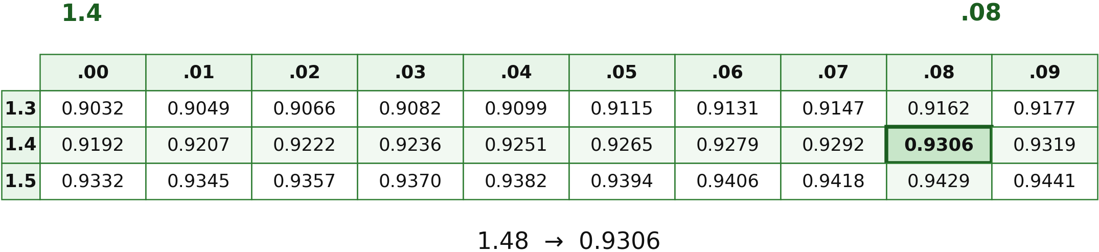
The table gives

\[\Phi(1.48)=0.9306.\]

Therefore,

\[P(Z<1.48)=0.9306.\]

A negative value is read in the same way if the table includes negative \(z\)-scores. For example,

\[\Phi(-0.25)=0.4013,\]

so

\[P(Z<-0.25)=0.4013.\]

4.4.7 Three Basic Probability Patterns

Most standard-normal calculations reduce to three patterns.

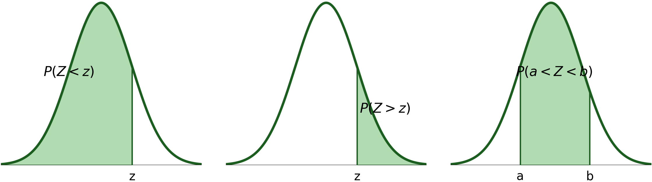
Pattern 1: Left of a value

\[P(Z<z)=\Phi(z).\]

This is read directly from a cumulative table.

Pattern 2: Right of a value

The total area is 1, so

\[P(Z>z) = 1-\Phi(z).\]

Pattern 3: Between two values

For \(a<b\),

\[P(a<Z<b) = \Phi(b)-\Phi(a).\]

The same rules work whether \(a\) and \(b\) are positive, negative, or on opposite sides of zero.

4.4.8 Example: Left-Tail Probability

Find

\[P(Z<1.48).\]

From the table,

\[\Phi(1.48)=0.9306.\]

Therefore,

\[P(Z<1.48)=0.9306.\]

Interpretation: about 93.06% of the standard normal area lies to the left of \(z=1.48\).

4.4.9 Example: Right-Tail Probability

Find

\[P(Z>1.60).\]

The table gives

\[\Phi(1.60)=0.9452.\]

Use the complement:

\[P(Z>1.60) = 1-P(Z<1.60)\]

\[=1-0.9452 =0.0548.\]

A right-tail probability for a positive \(z\) should be relatively small, which is consistent with this answer.

Now consider

\[P(Z>-1.02).\]

From the table,

\[\Phi(-1.02)=0.1539.\]

Therefore,

\[P(Z>-1.02) = 1-0.1539 = 0.8461.\]

4.4.10 Example: Probability Between Two z-Scores

Find

\[P(0.50<Z<1.57).\]

From the cumulative table,

\[\Phi(0.50)=0.6915\]

and

\[\Phi(1.57)=0.9418.\]

Therefore,

\[P(0.50<Z<1.57) = \Phi(1.57)-\Phi(0.50)\]

\[=0.9418-0.6915 =0.2503.\]

The same procedure works if the interval crosses zero.

For example,

\[P(-2.55<Z<0.09) = \Phi(0.09)-\Phi(-2.55).\]

Using

\[\Phi(0.09)=0.5359\]

and

\[\Phi(-2.55)=0.0054,\]

we obtain

\[P(-2.55<Z<0.09) = 0.5359-0.0054 =0.5305.\]

4.4.11 Symmetry of the Standard Normal Curve

The standard normal curve is symmetric about zero.

Therefore,

\[\Phi(-z)=1-\Phi(z).\]

Equivalently,

\[P(Z<-z)=P(Z>z).\]

For example,

\[P(Z<-1.08)=P(Z>1.08).\]

Symmetry is especially useful if a table contains only positive \(z\)-scores.

Another useful result is

\[P(-a<Z<a) = 2\Phi(a)-1.\]

The probability outside a symmetric interval is

\[P(Z<-a\text{ or }Z>a) = 2[1-\Phi(a)].\]

For example, since

\[\Phi(1.96)\approx0.9750,\]

we obtain

\[P(-1.96<Z<1.96) \approx 0.9500\]

and

\[P(Z<-1.96\text{ or }Z>1.96) \approx 0.0500.\]

These values will appear frequently in later statistical inference topics.

4.4.12 Very Large Positive or Negative z-Scores

Some printed tables stop near \(z=3.5\) or \(z=4.0\).

If \(z\) is far to the right, then

\[\Phi(z)\approx1.\]

If \(z\) is far to the left, then

\[\Phi(z)\approx0.\]

For example,

\[\Phi(4.16)\approx1.0000\]

when rounded to four decimal places.

Thus,

\[P(1.13<Z<4.16) \approx 1.0000-0.8708 =0.1292.\]

Likewise,

\[\Phi(-5.22)\approx0.0000.\]

These approximations reflect extremely small tail areas.

4.4.13 From a Probability Back to a z-Score

Sometimes the probability is known and the corresponding \(z\)-value is unknown.

Suppose

\[\Phi(z)=0.9500.\]

Search the body of the cumulative table for a value near \(0.9500\) and read the corresponding row and column.

This gives approximately

\[z\approx1.645.\]

Similarly,

\[\Phi(z)=0.9750\]

corresponds to

\[z\approx1.96.\]

This reverse lookup is the basis for finding critical values and percentiles later in the course.

4.4.14 Training with z-Scores Before Probability

Before using a probability table, be comfortable interpreting the standardized scale itself.

Suppose a measurement has

\[\mu=50, \qquad \sigma=6.\]

Then:

\(x\)	\(z\)	Interpretation
50	0	at the mean
56	1	one standard deviation above the mean
44	-1	one standard deviation below the mean
62	2	two standard deviations above the mean
38	-2	two standard deviations below the mean

For example,

\[z = \frac{62-50}{6} =2.\]

The value 62 is therefore two standard deviations above the mean.

This interpretation does not require a probability calculation.

4.4.15 A Reliable Workflow for Standard Normal Problems

When working with \(Z\), use the following procedure.

1. Identify the requested region.

   Decide whether the probability is left of, right of, between, or outside specified \(z\)-values.

2. Sketch the region mentally or on paper.

   This helps determine whether the answer should be small or large.

3. Read cumulative probabilities.

   Use

   \[\Phi(z)=P(Z<z).\]

4. Apply the appropriate probability rule.

   • left tail: \(\Phi(z)\);

   • right tail: \(1-\Phi(z)\);

   • interval: \(\Phi(b)-\Phi(a)\);

   • symmetric tails: use symmetry when helpful.

5. Check the answer.

   A probability must lie between 0 and 1 and should agree with the shaded region you intended to calculate.

4.4.16 Quick Practice

Use a cumulative standard normal table or software.

1. Find

\[P(Z<-1.72).\]

2. Find

\[P(Z>1.63).\]

3. Find

\[P(-0.93<Z<0.55).\]

4. Find

\[P(Z<-1.96\text{ or }Z>1.96).\]

5. A value is \(1.5\) standard deviations below its mean. What is its \(z\)-score?

6. A measurement has \(\mu=80\) and \(\sigma=5\). Find the \(z\)-score of \(x=92\).

Answers

1. \[P(Z<-1.72)=0.0427.\]
2. \[P(Z>1.63) = 1-0.9484 =0.0516.\]
3. \[P(-0.93<Z<0.55) = 0.7088-0.1762 =0.5326.\]
4. \[P(Z<-1.96\text{ or }Z>1.96) \approx0.0500.\]
5. \[z=-1.5.\]
6. \[z = \frac{92-80}{5} =2.4.\]

4.4.17 Common Mistakes

Mistake 1: Reversing the numerator

Use

\[z=\frac{x-\mu}{\sigma},\]

not \((\mu-x)/\sigma\).

Mistake 2: Ignoring the sign of z

A negative \(z\) is below the mean. A positive \(z\) is above the mean.

Mistake 3: Treating a cumulative table as a right-tail table

If the table gives \(\Phi(z)=P(Z<z)\), a right-tail probability requires

\[1-\Phi(z).\]

Mistake 4: Adding instead of subtracting for an interval

For \(a<b\),

\[P(a<Z<b) = \Phi(b)-\Phi(a).\]

Mistake 5: Worrying about < versus <=

Because \(Z\) is continuous,

\[P(Z<z)=P(Z\leq z).\]

Mistake 6: Assuming every z-score follows the standard normal distribution

A \(z\)-score is a standardized position. Additional distributional information is required before standard normal probabilities can be attached to an arbitrary standardized variable.

4.4.18 Summary

A \(z\)-score converts distance from the mean into standard deviation units:

\[z=\frac{x-\mu}{\sigma}.\]

The standard normal reference variable has

\[Z\sim N(0,1),\]

with mean 0 and standard deviation 1.

Its cumulative distribution function is

\[\Phi(z)=P(Z<z).\]

The main probability rules are

\[P(Z<z)=\Phi(z),\]

\[P(Z>z)=1-\Phi(z),\]

and

\[P(a<Z<b)=\Phi(b)-\Phi(a).\]

Symmetry gives

\[\Phi(-z)=1-\Phi(z).\]

The key skill from this section is to become comfortable thinking on the z-scale and translating shaded regions into cumulative probabilities.

In the next section, we will use this standard reference scale to work with the general normal distribution.