4.2 Continuous Uniform Distribution

4.2.1 From Discrete to Continuous Uniform

The uniform idea means that probability is spread evenly across the possible range.

For a discrete uniform random variable, individual values can have positive probability. If there are \(n\) equally likely values,

\[P(X=x_i)=\frac1n.\]

For a continuous uniform random variable, there are infinitely many possible values in an interval. An individual point therefore has probability zero:

\[P(X=x)=0.\]

Instead of assigning probability to individual points, a continuous model assigns probability through area under a probability density function. Equal-length subintervals have equal probability.

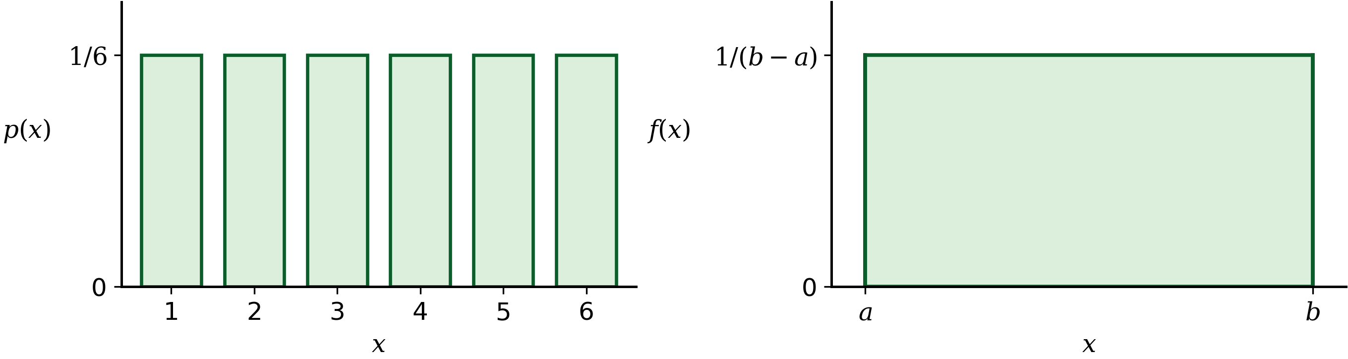
The figure shows the conceptual transition. The discrete model places equal probability masses at separate values, whereas the continuous model spreads density uniformly across an entire interval.

4.2.2 Probability Density Function

Let

\[X\sim U(a,b), \qquad a<b.\]

Then \(X\) can take any real value between \(a\) and \(b\), and its probability density function is

Note

Continuous Uniform PDF

\[\begin{split}f(x) = \begin{cases} \dfrac{1}{b-a}, & a\leq x\leq b,\\[6pt] 0, & \text{otherwise}. \end{cases}\end{split}\]

The graph is a rectangle over \([a,b]\). Its width is

\[b-a,\]

and its height is

\[\frac1{b-a}.\]

The height is determined by the requirement that the total probability be 1:

\[\int_{-\infty}^{\infty}f(x)\,dx = \int_a^b\frac1{b-a}\,dx = \frac{b-a}{b-a} =1.\]

Therefore, if the interval becomes wider, the density must become lower. If the interval becomes narrower, the density becomes higher.

Important

Density height is not the probability of an exact value. For a continuous random variable,

\[f(x)\neq P(X=x), \qquad P(X=x)=0.\]

4.2.3 Probability as Area and Interval Length

Suppose

\[a\leq c<d\leq b.\]

Then

\[\begin{split}\begin{aligned} P(c\leq X\leq d) &=\int_c^d f(x)\,dx\\ &=\int_c^d\frac1{b-a}\,dx\\ &=\frac{d-c}{b-a}. \end{aligned}\end{split}\]

Thus,

Note

Probability = favorable interval length / total interval length

\[\boxed{ P(c\leq X\leq d) = \frac{d-c}{b-a} }\]

This is the continuous analogue of the equally likely counting rule. For a discrete uniform distribution we compare counts; for a continuous uniform distribution we compare lengths.

Because a single point has probability zero, including or excluding an endpoint does not change an interval probability. For example,

\[P(c<X<d) =P(c\leq X<d) =P(c<X\leq d) =P(c\leq X\leq d).\]

4.2.4 Example: Electric Current in a Copper Wire

Let \(X\) represent current, in milliamperes, measured in a thin copper wire. Suppose

\[X\sim U(4.9,5.1).\]

The width of the interval is

\[5.1-4.9=0.2,\]

so the density is

\[f(x)=\frac1{0.2}=5, \qquad 4.9\leq x\leq5.1.\]

Find the probability that the current is between \(4.95\) and \(5.00\) mA.

\[\begin{split}\begin{aligned} P(4.95\leq X\leq5.00) &=\int_{4.95}^{5.00}5\,dx\\ &=5(5.00-4.95)\\ &=5(0.05)\\ &=0.25. \end{aligned}\end{split}\]

Equivalently, using interval lengths,

\[P(4.95\leq X\leq5.00) = \frac{5.00-4.95}{5.10-4.90} = \frac{0.05}{0.20} =0.25.\]

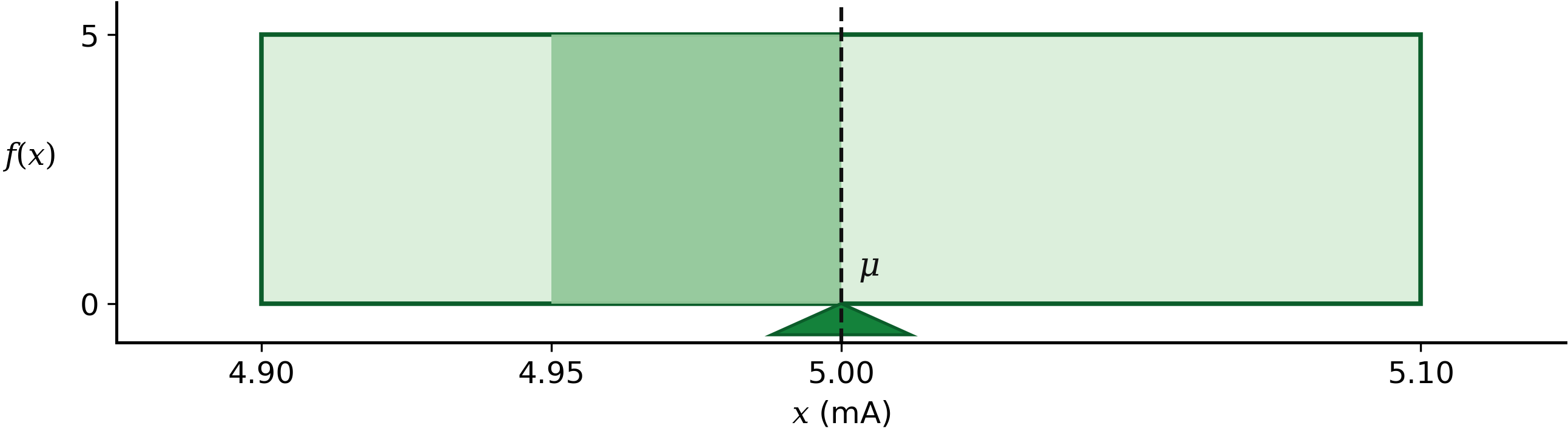
The shaded portion is one quarter of the total rectangle, so its area—and therefore its probability—is \(0.25\). The triangular support indicates the balance point of the uniform density, which will also be its mean.

4.2.5 Cumulative Distribution Function

The cumulative distribution function is

\[F(x)=P(X\leq x).\]

For \(X\sim U(a,b)\), consider three regions.

If \(x<a\), no probability has accumulated:

\[F(x)=0.\]

If \(a\leq x<b\), integrate from the left endpoint to \(x\):

\[\begin{split}\begin{aligned} F(x) &=\int_a^x\frac1{b-a}\,dt\\ &=\frac{x-a}{b-a}. \end{aligned}\end{split}\]

If \(x\geq b\), the entire probability has accumulated:

\[F(x)=1.\]

Therefore,

Note

Continuous Uniform CDF

\[\begin{split}F(x) = \begin{cases} 0, & x<a,\\[4pt] \dfrac{x-a}{b-a}, & a\leq x<b,\\[8pt] 1, & x\geq b. \end{cases}\end{split}\]

Inside \([a,b]\), the CDF increases linearly because equal increases in \(x\) add equal amounts of probability.

4.2.6 Deriving the Mean

For any continuous random variable,

\[E(X)=\int_{-\infty}^{\infty}x f(x)\,dx.\]

For \(X\sim U(a,b)\), the density is zero outside \([a,b]\), so

\[\begin{split}\begin{aligned} E(X) &=\int_a^b x\frac1{b-a}\,dx\\ &=\frac1{b-a}\int_a^b x\,dx\\ &=\frac1{b-a}\left[\frac{x^2}{2}\right]_a^b\\ &=\frac{b^2-a^2}{2(b-a)}. \end{aligned}\end{split}\]

Since

\[b^2-a^2=(b-a)(a+b),\]

we obtain

\[\boxed{ E(X)=\mu=\frac{a+b}{2} }.\]

The mean is the midpoint of the interval. This also follows from symmetry: the probability mass is balanced equally on both sides of the midpoint.

For the electric-current example,

\[E(X) = \frac{4.9+5.1}{2} =5.0\text{ mA}.\]

4.2.7 Deriving the Variance and Standard Deviation

The variance is the expected squared distance from the mean:

\[\operatorname{Var}(X) = E[(X-\mu)^2].\]

For the continuous uniform distribution,

\[\operatorname{Var}(X) = \int_a^b \left(x-\frac{a+b}{2}\right)^2 \frac1{b-a}\,dx.\]

Let

\[\mu=\frac{a+b}{2}, \qquad h=\frac{b-a}{2},\]

and set

\[u=x-\mu.\]

When \(x=a\), \(u=-h\); when \(x=b\), \(u=h\). Also, \(b-a=2h\). Therefore,

\[\begin{split}\begin{aligned} \operatorname{Var}(X) &=\frac1{2h}\int_{-h}^{h}u^2\,du\\ &=\frac1{2h}\left[\frac{u^3}{3}\right]_{-h}^{h}\\ &=\frac1{2h}\left(\frac{h^3}{3}+\frac{h^3}{3}\right)\\ &=\frac{h^2}{3}. \end{aligned}\end{split}\]

Substituting \(h=(b-a)/2\),

\[\boxed{ \operatorname{Var}(X) = \frac{(b-a)^2}{12} }.\]

The standard deviation is

\[\boxed{ \sigma = \frac{b-a}{\sqrt{12}} }.\]

A useful consequence is that the variance depends only on the width of the interval, not on its location.

For the electric-current example,

\[\begin{split}\begin{aligned} \operatorname{Var}(X) &=\frac{(5.1-4.9)^2}{12}\\ &=\frac{0.04}{12}\\ &\approx0.00333\text{ mA}^2, \end{aligned}\end{split}\]

and

\[\sigma =\sqrt{0.00333} \approx0.0577\text{ mA}.\]

4.2.8 Percentiles and the Inverse CDF

A percentile is particularly simple for a continuous uniform distribution. Let \(k\) be the value below which a proportion \(r\) of the probability lies, where \(0<r<1\). Then

\[F(k)=r.\]

Inside \([a,b]\),

\[\frac{k-a}{b-a}=r.\]

Solving for \(k\),

\[\boxed{ k=a+r(b-a) }.\]

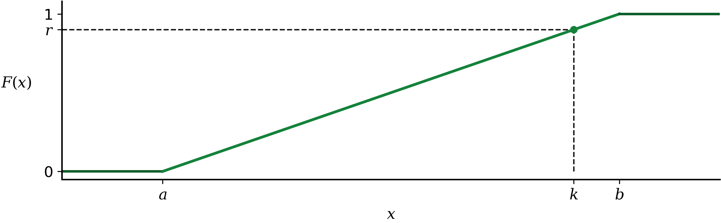
For example, if waiting time is uniformly distributed from 0 to 15 minutes, then the 90th percentile is

\[k =0+0.90(15) =13.5\text{ minutes}.\]

Thus, 90% of waiting times are at most 13.5 minutes.

The 50th percentile is

\[a+0.50(b-a) =\frac{a+b}{2},\]

which is also the mean and median because the distribution is symmetric.

4.2.9 Conditional Probability on a Reduced Interval

Uniform distributions also make some conditional probabilities easy to interpret geometrically.

Suppose

\[a\leq c<d\leq b.\]

If we already know that \(X>c\), the relevant interval has been reduced from \([a,b]\) to \((c,b]\). Therefore,

\[\begin{split}\begin{aligned} P(X>d\mid X>c) &=\frac{P(X>d)}{P(X>c)}\\ &=\frac{(b-d)/(b-a)}{(b-c)/(b-a)}\\ &=\frac{b-d}{b-c}. \end{aligned}\end{split}\]

So after conditioning on \(X>c\), probability is again proportional to length within the reduced interval.

4.2.10 Discrete Uniform Versus Continuous Uniform

Feature	Discrete Uniform	Continuous Uniform
Possible outcomes	Finite or countable values	All real values in an interval
Probability model	PMF \(p(x)\)	PDF \(f(x)\)
Probability at one value	Can be positive	\(P(X=x)=0\)
Probability over a range	Sum of probability masses	Area under the density
Graph	Equal-height bars or spikes	Rectangle
Uniform idea	Equal probability for each value	Equal probability for equal-length intervals

The phrase equally likely must therefore be interpreted differently in the two settings. In a continuous interval, it means equal lengths have equal probability; it does not mean that each exact real number has positive probability.

4.2.11 When Is a Continuous Uniform Model Appropriate?

Use a continuous uniform model when:

1. the variable is continuous;

2. values are restricted to a finite interval \([a,b]\);

3. no part of the interval is more likely than another;

4. equal-length subintervals should have equal probability.

Examples can include randomized waiting times, measurement values known only to lie uniformly inside a tolerance interval, or a random location along a fixed line segment.

Do not use a uniform model if values near the center, near an endpoint, or in some other part of the interval are systematically more likely.

4.2.12 Quick Practice

Suppose a service time is uniformly distributed between 11 and 21 minutes. Let

\[X\sim U(11,21).\]

Find:

1. \(P(X>19)\);

2. the 50th percentile;

3. \(E(X)\); and

4. \(\sigma\).

Answer

The full interval has width

\[21-11=10.\]

For part (a),

\[P(X>19) =\frac{21-19}{10} =0.20.\]

For part (b),

\[k =11+0.50(10) =16.\]

The mean is

\[E(X) =\frac{11+21}{2} =16.\]

The standard deviation is

\[\sigma =\frac{10}{\sqrt{12}} \approx2.887\text{ minutes}.\]

4.2.13 Common Mistakes

Do not interpret \(f(x)\) as \(P(X=x)\). A continuous point has zero probability.

Do not divide by \(b\). The total interval length is \(b-a\).

Do not forget to rescale the density if the interval changes. The total area must always remain 1.

Do not treat endpoints as extra probability masses. For continuous probabilities, including or excluding a finite number of endpoints does not change the probability.

Do not use the uniform model merely because the variable is bounded. The model also requires a constant density across the interval.

4.2.14 Summary

For

\[X\sim U(a,b),\]

its PDF is

\[f(x) = \frac1{b-a}, \qquad a\leq x\leq b.\]

For \(a\leq c<d\leq b\),

\[P(c\leq X\leq d) = \frac{d-c}{b-a}.\]

The CDF is

\[\begin{split}F(x) = \begin{cases} 0, & x<a,\\[4pt] \dfrac{x-a}{b-a}, & a\leq x<b,\\[8pt] 1, & x\geq b. \end{cases}\end{split}\]

The mean, variance, and standard deviation are

\[E(X)=\frac{a+b}{2}, \qquad \operatorname{Var}(X)=\frac{(b-a)^2}{12}, \qquad \sigma=\frac{b-a}{\sqrt{12}}.\]

The central idea is:

probability is represented by area, and equal-length intervals have equal probability.