4.3 Exponential Distribution

4.3.1 Main Idea

The exponential distribution models a continuous waiting time until the next event occurs when events arise independently at a constant average rate.

It is closely connected to the Poisson process:

• the Poisson distribution counts how many events occur in a fixed interval;

• the exponential distribution measures how long we wait until the next event.

Typical examples include:

• time until the next customer arrives;

• time between telephone calls;

• distance until the next flaw appears;

• lifetime of a component when its failure rate is constant.

Let

\[\lambda>0\]

be the event rate per unit time or space. If \(X\) denotes the waiting time until the next event, then

\[X\geq0.\]

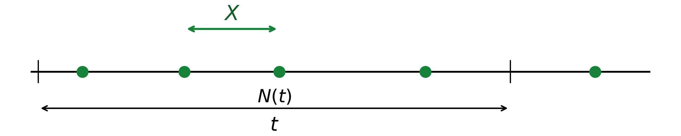
The same event process can therefore be viewed in two ways. Over a fixed interval, we may count events. Starting from one event, we may instead measure the continuous distance or time to the next event.

4.3.2 Rate and Mean-Waiting-Time Parameterizations

Two equivalent parameterizations are commonly used.

If \(\lambda\) is the event rate, then the mean waiting time is

\[\mu=\frac1\lambda.\]

Equivalently,

\[\lambda=\frac1\mu.\]

Some references use a symbol such as \(m\) for this rate or decay parameter. In this handout, we use \(\lambda\) consistently.

Thus the two equivalent forms of the density are

\[f(x)=\lambda e^{-\lambda x}\]

and

\[f(x)=\frac1\mu e^{-x/\mu}.\]

The units are important:

• \(\lambda\) has units of events per unit time;

• \(\mu\) and \(X\) have units of time.

For example, if customers arrive at an average rate of 30 per hour, then

\[\lambda=\frac{30}{60}=0.5\text{ per minute},\]

so the mean waiting time is

\[\mu=\frac1{0.5}=2\text{ minutes}.\]

4.3.3 Probability Density Function

A random variable \(X\) has an exponential distribution with rate \(\lambda\) if

Note

Exponential PDF

\[\begin{split}f(x) = \begin{cases} \lambda e^{-\lambda x}, & x\geq0,\\ 0, & x<0. \end{cases}\end{split}\]

The density is largest at \(x=0\):

\[f(0)=\lambda.\]

It then decreases continuously toward zero as \(x\) increases. This is why small waiting times are more common than very large waiting times.

As with every probability density function, the total area must equal 1:

\[\int_{-\infty}^{\infty}f(x)\,dx = \int_0^\infty \lambda e^{-\lambda x}\,dx.\]

Since

\[\int \lambda e^{-\lambda x}\,dx = -e^{-\lambda x},\]

we obtain

\[\int_0^\infty \lambda e^{-\lambda x}\,dx = \left[-e^{-\lambda x}\right]_0^\infty = 0-(-1) =1.\]

The value \(f(x)\) is a density, not the probability of one exact waiting time. Because \(X\) is continuous,

\[P(X=x)=0.\]

4.3.4 CDF and Survival Function

The cumulative distribution function is

\[F(x)=P(X\leq x).\]

For \(x\geq0\), integrate the density from 0 to \(x\):

\[F(x) = \int_0^x \lambda e^{-\lambda t}\,dt.\]

Therefore,

\[F(x) = \left[-e^{-\lambda t}\right]_0^x = 1-e^{-\lambda x}.\]

Hence,

Note

Exponential CDF

\[\begin{split}F(x) = \begin{cases} 0, & x<0,\\ 1-e^{-\lambda x}, & x\geq0. \end{cases}\end{split}\]

The complementary probability

\[P(X>x)\]

is called the survival function. It is

\[P(X>x) = 1-F(x) = e^{-\lambda x}.\]

This simple exponential tail is one of the most useful properties of the distribution.

4.3.5 Probability Calculations

For \(x\geq0\),

\[P(X\leq x) = 1-e^{-\lambda x}.\]

For waiting more than \(x\),

\[P(X>x) = e^{-\lambda x}.\]

For an interval \(0\leq a<b\),

\[P(a<X<b) = F(b)-F(a).\]

Substituting the exponential CDF gives

\[P(a<X<b) = e^{-\lambda a}-e^{-\lambda b}.\]

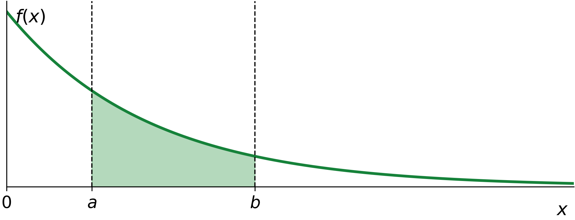
The shaded area under the density between two time points represents the probability that the event occurs during that waiting-time interval.

Because \(X\) is continuous, endpoint inclusion does not matter:

\[P(a<X<b) = P(a\leq X\leq b).\]

4.3.6 Main Example: Time Between Customer Arrivals

Suppose customers arrive according to a Poisson process at an average rate of 30 customers per hour.

Express the rate in minutes:

\[\lambda=\frac{30}{60}=0.5\text{ per minute}.\]

Let

\[X=\text{time in minutes until the next customer arrives}.\]

Then

\[X\sim\operatorname{Exp}(0.5).\]

The mean waiting time is

\[E(X)=\frac1{0.5}=2\text{ minutes}.\]

Probability that the next customer arrives within one minute

\[P(X<1) = 1-e^{-0.5(1)} \approx0.3935.\]

Probability that the wait exceeds five minutes

\[P(X>5) = e^{-0.5(5)} = e^{-2.5} \approx0.0821.\]

Probability that the waiting time is between one and three minutes

\[P(1<X<3) = e^{-0.5(1)}-e^{-0.5(3)} \approx0.3834.\]

These three calculations illustrate the three common forms of exponential probability questions: left-tail, right-tail, and interval probabilities.

4.3.7 Deriving the Mean

For a continuous random variable,

\[E(X) = \int_{-\infty}^{\infty}x f(x)\,dx.\]

For an exponential random variable,

\[E(X) = \int_0^\infty x\lambda e^{-\lambda x}\,dx.\]

Use integration by parts. Let

\[u=x, \qquad dv=\lambda e^{-\lambda x}\,dx.\]

Then

\[du=dx, \qquad v=-e^{-\lambda x}.\]

Therefore,

\[E(X) = \left[-xe^{-\lambda x}\right]_0^\infty + \int_0^\infty e^{-\lambda x}\,dx.\]

The boundary term is zero, so

\[E(X) = \left[-\frac1\lambda e^{-\lambda x}\right]_0^\infty = \frac1\lambda.\]

Thus,

Note

Mean of an Exponential Distribution

\[\boxed{E(X)=\mu=\frac1\lambda}.\]

A larger event rate therefore produces a shorter mean waiting time.

4.3.8 Deriving the Variance and Standard Deviation

Use

\[\operatorname{Var}(X) = E(X^2)-[E(X)]^2.\]

First compute

\[E(X^2) = \int_0^\infty x^2\lambda e^{-\lambda x}\,dx.\]

Again use integration by parts with

\[u=x^2, \qquad dv=\lambda e^{-\lambda x}\,dx.\]

Then

\[du=2x\,dx, \qquad v=-e^{-\lambda x}.\]

Therefore,

\[E(X^2) = \left[-x^2e^{-\lambda x}\right]_0^\infty + 2\int_0^\infty x e^{-\lambda x}\,dx.\]

The boundary term is zero. Also,

\[\int_0^\infty x e^{-\lambda x}\,dx = \frac1{\lambda^2}.\]

Hence,

\[E(X^2)=\frac2{\lambda^2}.\]

Now

\[\operatorname{Var}(X) = \frac2{\lambda^2} - \left(\frac1\lambda\right)^2 = \frac1{\lambda^2}.\]

Therefore,

Note

Variance and Standard Deviation

\[\boxed{\operatorname{Var}(X)=\frac1{\lambda^2}}\]

and

\[\boxed{\sigma=\frac1\lambda}.\]

Thus, for an exponential distribution,

\[\boxed{\sigma=\mu}.\]

The mean and standard deviation have the same numerical value and the same units.

4.3.9 Percentiles and the Median

Suppose \(k_r\) is the \(r\)-th percentile, where \(0<r<1\). Then

\[P(X\leq k_r)=r.\]

Using the CDF,

\[1-e^{-\lambda k_r}=r.\]

Therefore,

\[e^{-\lambda k_r}=1-r.\]

Take natural logarithms:

\[-\lambda k_r = \ln(1-r).\]

Hence,

Note

Exponential Percentile

\[\boxed{ k_r=-\frac{\ln(1-r)}{\lambda} }.\]

For the median, \(r=0.50\), so

\[k_{0.50} = \frac{\ln2}{\lambda} \approx \frac{0.6931}{\lambda}.\]

Because

\[\frac{\ln2}{\lambda} < \frac1\lambda,\]

we have

\[\text{median}<\text{mean}.\]

This is consistent with the right-skewed shape of the exponential distribution.

For the customer-arrival example, \(\lambda=0.5\). The 70th percentile is

\[k_{0.70} = -\frac{\ln(0.30)}{0.5} \approx2.41\text{ minutes}.\]

Thus, 70% of the waiting times are at most about 2.41 minutes.

4.3.10 Memoryless Property

The exponential distribution is memoryless. For \(s,t\geq0\),

\[P(X>s+t\mid X>s) = P(X>t).\]

To see why, use conditional probability:

\[P(X>s+t\mid X>s) = \frac{P(X>s+t)}{P(X>s)}.\]

Using the survival function,

\[P(X>s+t\mid X>s) = \frac{e^{-\lambda(s+t)}}{e^{-\lambda s}} = e^{-\lambda t}.\]

But

\[e^{-\lambda t}=P(X>t).\]

Therefore,

\[\boxed{ P(X>s+t\mid X>s)=P(X>t) }.\]

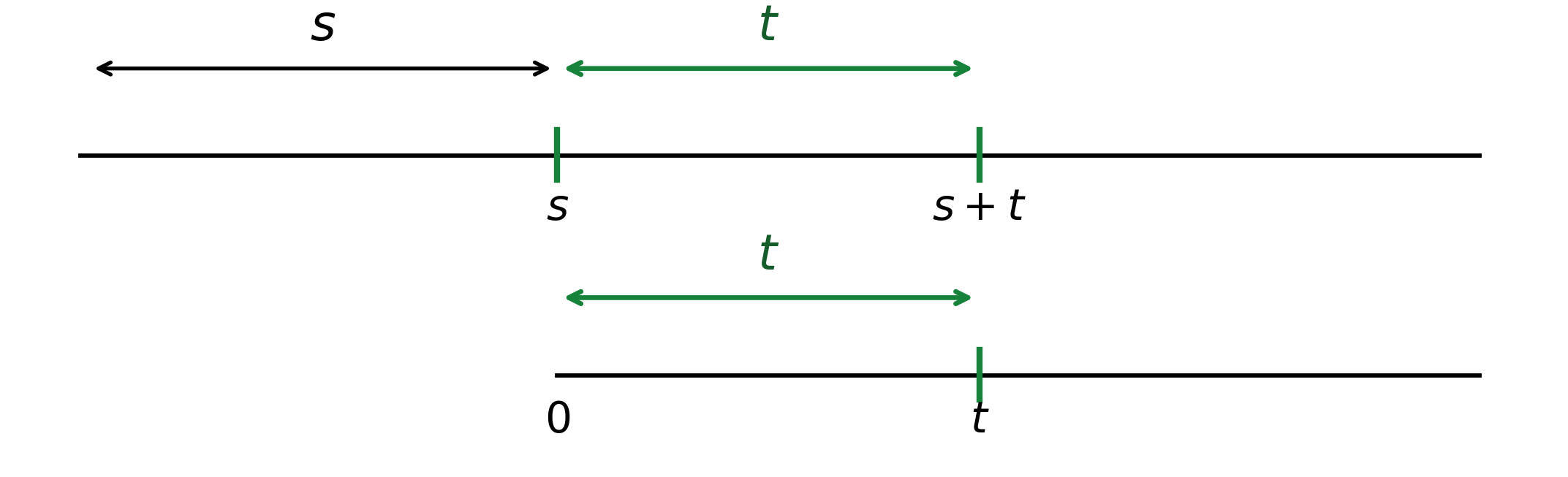
For the customer-arrival example, suppose 5 minutes have already passed with no arrival. The probability of waiting more than one additional minute is still

\[P(X>1) = e^{-0.5} \approx0.6065.\]

The previous five minutes do not make an arrival “due.”

4.3.11 Connection to the Poisson Distribution

The Poisson and exponential distributions describe the same underlying event process from two different perspectives.

Suppose events follow a Poisson process with rate \(\lambda\), and let

\[N(t)=\text{number of events during an interval of length }t.\]

Then

\[N(t)\sim\operatorname{Poisson}(\lambda t).\]

Let

\[T=\text{waiting time until the first event}.\]

The event

\[T>t\]

means that no event has occurred by time \(t\). Therefore,

\[P(T>t) = P(N(t)=0).\]

Using the Poisson PMF,

\[P(N(t)=0) = \frac{e^{-\lambda t}(\lambda t)^0}{0!} = e^{-\lambda t}.\]

Thus,

\[P(T>t)=e^{-\lambda t}.\]

Therefore,

\[F_T(t) = 1-e^{-\lambda t}.\]

Differentiating gives

\[f_T(t) = \lambda e^{-\lambda t}.\]

This is exactly the exponential distribution.

So:

Poisson -> number of events in a fixed interval.

Exponential -> waiting time until the next event.

4.3.12 Reliability Interpretation and Constant Hazard

The exponential distribution is often used in reliability when the failure rate is approximately constant.

The hazard rate is

\[h(x) = \frac{f(x)}{P(X>x)}.\]

For an exponential random variable,

\[h(x) = \frac{\lambda e^{-\lambda x}}{e^{-\lambda x}} = \lambda.\]

Thus the hazard is constant over time.

For example, suppose a component lifetime is exponential with mean 10 years. Then

\[\lambda=\frac1{10}=0.1\text{ per year}.\]

The probability that it survives more than 7 years is

\[P(X>7) = e^{-0.1(7)} \approx0.4966.\]

This model is appropriate only when a constant failure rate is plausible. It is not suitable for strong wear-out or aging behavior in which failure risk increases with age.

4.3.13 Exponential, Poisson, and Geometric

Feature	Exponential	Poisson	Geometric
Type	Continuous	Discrete	Discrete
Random variable	Waiting time	Event count	Number of trials until success
Typical setting	Continuous event process	Continuous event process	Repeated Bernoulli trials
Memoryless	Yes	Not applicable in this form	Yes

The exponential distribution can be viewed as the continuous analogue of the geometric waiting-time model. Both are memoryless, but one measures continuous time while the other counts discrete trials.

4.3.14 A Simple Method

For an exponential problem:

1. Define what \(X\) measures and identify its units.

2. Identify the event rate \(\lambda\), or convert from the mean using \(\lambda=1/\mu\).

3. Make the units of \(x\) compatible with the units of \(\lambda\).

4. Translate the probability statement:

   • less than -> use \(1-e^{-\lambda x}\);

   • more than -> use \(e^{-\lambda x}\);

   • between -> subtract two CDF values.

5. Interpret the result in the original context.

4.3.15 Quick Practice

Calls arrive at a service desk according to a Poisson process at an average rate of 4 calls per hour.

Let \(X\) be the waiting time in hours until the next call.

Find:

1. \(P(X>0.5)\);

2. \(P(X<0.25)\);

3. \(E(X)\); and

4. the median waiting time.

Answer

Here,

\[\lambda=4.\]

For part (a),

\[P(X>0.5) = e^{-4(0.5)} = e^{-2} \approx0.1353.\]

For part (b),

\[P(X<0.25) = 1-e^{-4(0.25)} = 1-e^{-1} \approx0.6321.\]

For part (c),

\[E(X)=\frac14\text{ hour}=15\text{ minutes}.\]

For part (d),

\[k_{0.50} = \frac{\ln2}{4}\text{ hour} \approx0.1733\text{ hour} \approx10.4\text{ minutes}.\]

4.3.16 Common Mistakes

A common mistake is to confuse the rate with the mean waiting time.

\[\mu=\frac1\lambda,\]

not \(\mu=\lambda\).

Another mistake is to use inconsistent units. If \(\lambda\) is measured per hour, then the waiting time inserted into the formula must be measured in hours.

A third mistake is to treat \(f(x)\) as a point probability. For a continuous random variable,

\[P(X=x)=0.\]

Another mistake is to use a Poisson PMF when the question asks how long until an event. Poisson counts events; exponential measures waiting time.

Finally, do not use the exponential model automatically for every lifetime. Its constant hazard rate excludes many aging and wear-out mechanisms.

4.3.17 Summary

For

\[X\sim\operatorname{Exp}(\lambda), \qquad \lambda>0,\]

with \(x\geq0\),

\[f(x)=\lambda e^{-\lambda x},\]

\[F(x)=1-e^{-\lambda x},\]

and

\[P(X>x)=e^{-\lambda x}.\]

The mean, variance, and standard deviation are

\[E(X)=\frac1\lambda,\]

\[\operatorname{Var}(X)=\frac1{\lambda^2},\]

and

\[\sigma=\frac1\lambda.\]

The \(r\)-th percentile is

\[k_r=-\frac{\ln(1-r)}{\lambda}.\]

The distribution is memoryless:

\[P(X>s+t\mid X>s) = P(X>t).\]

Its main connection to the Poisson distribution is:

Poisson counts events; exponential measures the waiting time between them.