2.4 Mean and Expected Value

Key Terms

Mean（平均數）

A numerical measure of the center of a probability distribution.

Expected value（期望值）

The probability-weighted average of a random variable.

Mathematical expectation（數學期望值）

Another term for expected value.

Weighted average（加權平均）

An average in which values with larger probabilities or densities have more influence.

Long-run average（長期平均）

The average approached over many repetitions of the same random experiment.

2.4.2 Learning Outcomes

After completing this section, students should be able to:

• explain the meaning of mean and expected value;

• calculate the expected value of a discrete random variable;

• calculate the expected value of a continuous random variable;

• interpret expected value as a probability-weighted balance point;

• explain why the mean need not be the midpoint of the possible range;

• explain why a discrete expected value need not be a possible outcome;

• distinguish expected value from an observed sample mean.

2.4.3 One Idea, Two Forms

The mean, or expected value, summarizes the location of a probability distribution.

For a discrete random variable with PMF \(p(x)\),

\[\mu=E(X)=\sum_x x\,p(x).\]

For a continuous random variable with PDF \(f(x)\),

\[\mu=E(X) = \int_{-\infty}^{\infty} x f(x)\,dx.\]

The idea is the same in both cases:

values with more probability have more influence on the mean.

For discrete variables, probability is concentrated at separate values, so we use a sum. For continuous variables, probability is distributed across an interval, so we use an integral.

2.4.4 Expected Value as a Balance Point

A useful physical interpretation is to imagine a thin beam placed along the possible values of \(X\).

For a discrete distribution, attach a weight at each possible value. The size of each weight is proportional to its probability.

The expected value is the point where the weighted beam balances.

This interpretation is useful because the balance point does not have to be the geometric center of the possible values.

2.4.5 Example 1: Uncertain Revenue

Suppose \(X\) is the revenue from a new product design, measured in millions of dollars.

The possible outcomes are

\(x\)	\(p(x)\)
2	0.70
7	0.30

The expected revenue is

\[E(X) = 2(0.70)+7(0.30) = 3.5.\]

The corresponding balance-point interpretation is shown below.

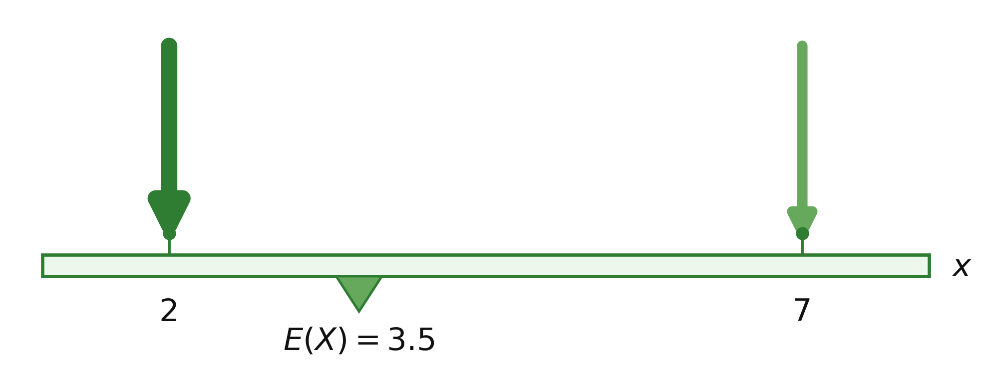
The midpoint between the two possible values is

\[\frac{2+7}{2}=4.5,\]

but the expected value is only \(3.5\) because the value 2 receives much more probability than the value 7.

Also notice that \(3.5\) is not a possible one-trial outcome. Revenue is either 2 or 7 million dollars in this simplified model.

Expected value describes the distribution as a whole; it does not have to be an outcome that can occur in one trial.

2.4.6 Expected Value as a Long-Run Average

Expected value also has a long-run interpretation.

If the same random experiment is repeated many times and the observed values are averaged, the average tends to approach \(E(X)\).

For the revenue example, individual outcomes are 2 or 7, but over many repetitions the average revenue would tend toward 3.5 million dollars.

Note

Expected value is a long-run average, not a prediction of the next individual outcome.

2.4.7 Continuous Expected Value

For a continuous distribution, we can use the same balance-point idea. Instead of separate probability weights, imagine probability density spread continuously along the beam.

Consider the density

\[\begin{split}f(x)= \begin{cases} 2(1-x), & 0\leq x\leq1,\\ 0, & \text{otherwise}. \end{cases}\end{split}\]

The density is larger near \(x=0\) and decreases toward \(x=1\).

Its expected value is

\[E(X) = \int_0^1 x\,2(1-x)\,dx = \frac13.\]

The continuous loading analogy is shown below.

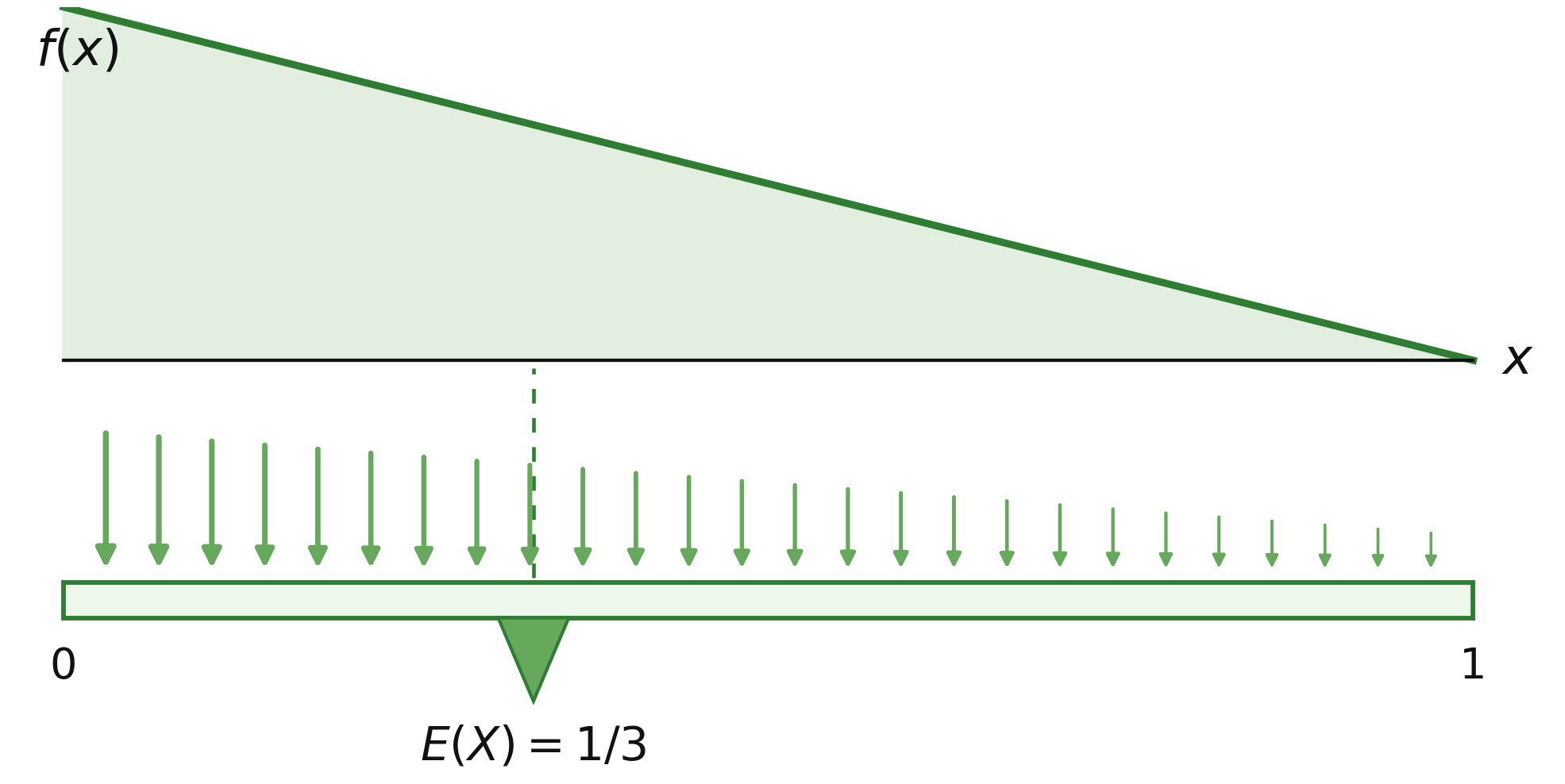
The geometric midpoint of the interval \([0,1]\) is \(1/2\), but

\[E(X)=\frac13.\]

The mean is shifted toward the left because more probability density is concentrated at smaller values.

This is why describing expected value simply as the “middle” can be misleading. A better interpretation is the probability-weighted center or balance point of the distribution.

2.4.8 Mean, Midpoint, and Most Likely Value

These ideas describe different features of a distribution.

The midpoint depends only on the endpoints of a range.

The most likely value depends on where probability or density is largest.

The expected value depends on the entire probability distribution.

Therefore, the expected value does not generally have to equal the midpoint or the most likely value.

2.4.9 Expected Value Versus Sample Mean

Expected value is a property of a probability model.

For a discrete random variable,

\[E(X)=\sum_x x\,p(x).\]

For a continuous random variable,

\[E(X)=\int_{-\infty}^{\infty}x f(x)\,dx.\]

A sample mean, by contrast, is calculated from observed data:

\[\bar{x} = \frac{x_1+x_2+\cdots+x_n}{n}.\]

The sample mean changes from sample to sample. The expected value is fixed by the probability distribution.

2.4.10 A Simple Method

For a discrete random variable:

1. List the possible values \(x\).

2. Write their probabilities \(p(x)\).

3. Calculate \(x\,p(x)\).

4. Add the products.

For a continuous random variable:

1. Identify the density \(f(x)\) and its range.

2. Form \(x f(x)\).

3. Integrate over the possible range.

Then interpret the result as a probability-weighted center or long-run average.

2.4.11 Common Mistakes

Do not calculate an ordinary unweighted average when probabilities differ.

Do not assume the expected value is the midpoint of the possible range.

Do not assume the expected value must be a possible discrete outcome.

Do not confuse expected value with the most likely value.

Do not interpret expected value as a guaranteed result from one trial.

2.4.12 Summary

Expected value is the probability-weighted center of a distribution.

For a discrete random variable,

\[E(X)=\sum_x x\,p(x).\]

For a continuous random variable,

\[E(X)=\int_{-\infty}^{\infty}x f(x)\,dx.\]

The same balance-point interpretation applies to both cases.

The expected value need not be the midpoint, the most likely value, or a possible one-trial outcome.