2.3 Continuous Probability Distributions

Key Terms

Probability density function（機率密度函數）

A function whose area over an interval gives probability.

PDF（機率密度函數）

Short form of probability density function.

Density（密度）

Probability concentration represented by height; probability itself is represented by area.

Cumulative distribution function（累積分配函數）

A function that gives the probability that a random variable is less than or equal to a given value.

CDF（累積分配函數）

Short form of cumulative distribution function.

Interval probability（區間機率）

Probability that a continuous random variable falls within an interval.

2.3.2 Learning Outcomes

After completing this section, students should be able to:

• explain why continuous probability is described by a PDF rather than a PMF;

• explain why \(P(X=x)=0\) for a continuous random variable;

• interpret probability as area under a density curve;

• identify the conditions of a valid PDF;

• calculate simple interval probabilities from a PDF;

• construct a CDF from a simple continuous PDF;

• use \(F(x)\) to calculate interval probabilities;

• explain the relationship between a PDF and a CDF;

• explain why including or excluding interval endpoints does not change a continuous probability.

2.3.3 From PMF to PDF

In the previous section, a discrete random variable was described by a probability mass function:

\[p(x)=P(X=x).\]

A discrete random variable can place positive probability at individual values.

A continuous random variable is different. Its possible values fill an interval, so probability is not assigned to individual points. Instead, a continuous distribution is described by a probability density function, or PDF.

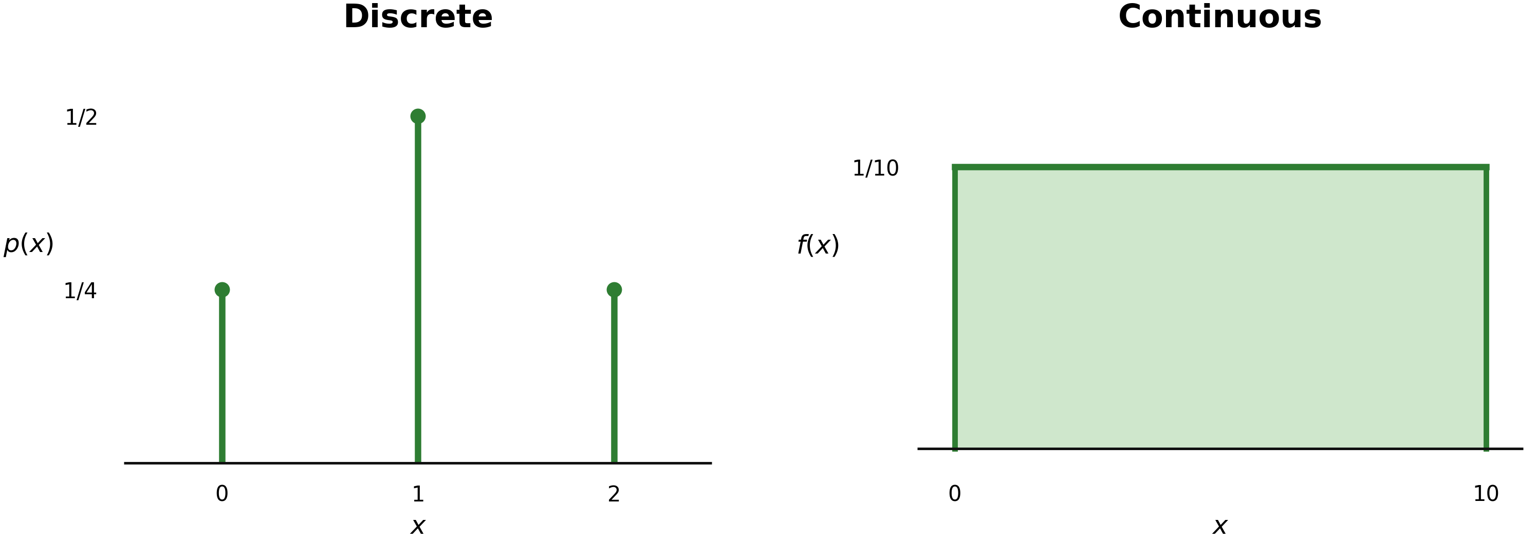
For a continuous random variable,

\[P(X=x)=0\]

for every individual value \(x\).

This does not mean that \(x\) is impossible. A single point has zero width, so it contributes zero area under the density curve.

Note

PMF versus PDF

For a discrete random variable,

\[p(x)=P(X=x).\]

For a continuous random variable,

\[f(x)\neq P(X=x).\]

Probability is obtained from area, not from the density height at one point.

2.3.4 A Single Example: Bus Waiting Time

Let \(X\) be the waiting time, in minutes, for the next bus.

Suppose the waiting time can be anywhere from 0 to 10 minutes and is modeled with the constant density

\[\begin{split}f(x)= \begin{cases} \frac{1}{10}, & 0\leq x\leq10,\\ 0, & \text{otherwise}. \end{cases}\end{split}\]

This one example will be used to introduce both the PDF and the CDF.

2.3.5 Probability Density Function

A valid PDF must satisfy two conditions:

\[f(x)\geq0\]

for all \(x\), and

\[\int_{-\infty}^{\infty}f(x)\,dx=1.\]

For the waiting-time example, the total area is

\[10\left(\frac{1}{10}\right)=1,\]

so the density is valid.

Probability over an interval is the area under the PDF:

\[P(a<X<b) = \int_a^b f(x)\,dx.\]

For example,

\[P(2<X<6) = \int_2^6 \frac{1}{10}\,dx = \frac{4}{10} = 0.40.\]

The corresponding area is shown below.

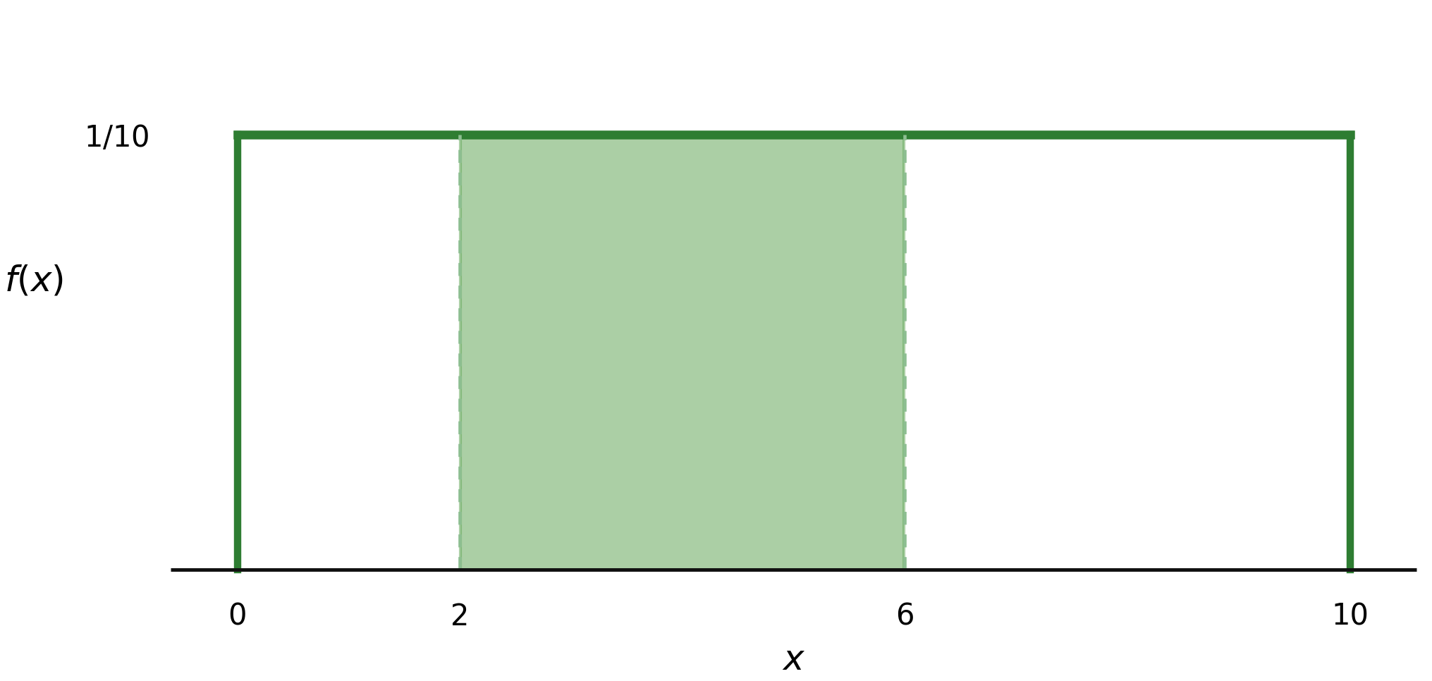
The height \(1/10\) is a density. The probability \(0.40\) comes from height multiplied by interval width.

2.3.6 Height Is Not Probability

For a continuous distribution,

\[f(x)\neq P(X=x).\]

In the waiting-time example,

\[f(4)=\frac{1}{10},\]

but

\[P(X=4)=0.\]

The density height describes how probability is concentrated near a value. Probability is obtained only after an interval has been specified.

A density value can even be greater than 1. This is allowed as long as the total area under the PDF is exactly 1.

2.3.7 Endpoints Do Not Matter

For a continuous random variable,

\[P(X=a)=P(X=b)=0.\]

Therefore,

\[P(a<X<b) = P(a\leq X<b) = P(a<X\leq b) = P(a\leq X\leq b).\]

For example,

\[P(2<X<6) = P(2\leq X\leq6) = 0.40.\]

The endpoints do not change the area and therefore do not change the probability.

2.3.8 Cumulative Distribution Function

The CDF is defined for both discrete and continuous random variables:

\[F(x)=P(X\leq x).\]

For a continuous random variable, the CDF is accumulated area under the PDF:

\[F(x) = \int_{-\infty}^{x}f(t)\,dt.\]

For the waiting-time example,

\[\begin{split}F(x)= \begin{cases} 0, & x<0,\\ \frac{x}{10}, & 0\leq x\leq10,\\ 1, & x>10. \end{cases}\end{split}\]

Thus,

\[F(2)=0.20, \qquad F(6)=0.60.\]

The CDF is shown below.

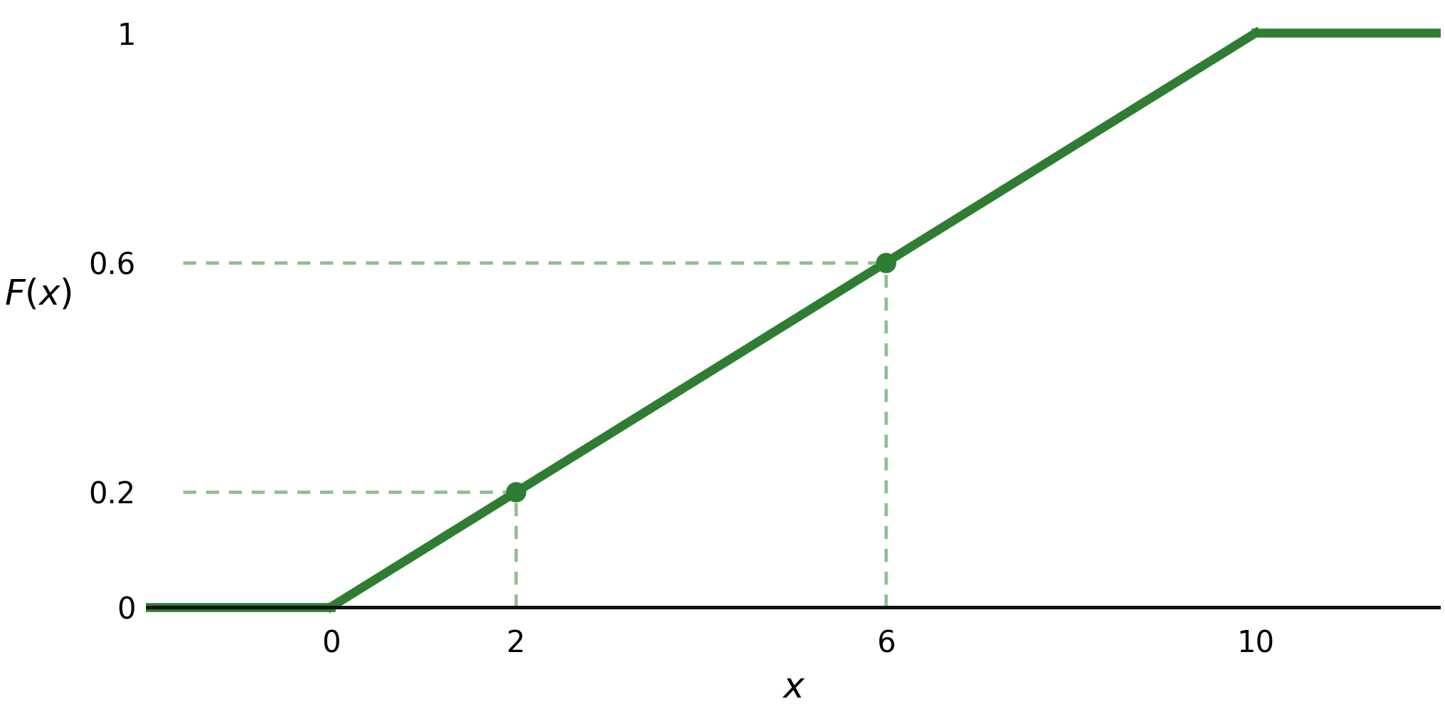
Unlike the discrete CDF, this CDF increases continuously rather than by jumps.

2.3.9 Finding Probabilities from the CDF

The CDF provides accumulated probability from the left.

For example,

\[P(X\leq6)=F(6)=0.60.\]

For an interval,

\[P(a<X<b)=F(b)-F(a).\]

Therefore,

\[P(2<X<6) = F(6)-F(2) = 0.60-0.20 = 0.40.\]

This is the same probability obtained earlier from the area under the PDF.

For an upper-tail probability,

\[P(X>x)=1-F(x).\]

For example,

\[P(X>6)=1-F(6)=0.40.\]

2.3.10 Relationship Between PDF and CDF

The PDF and CDF describe the same continuous distribution in different ways.

The CDF accumulates the PDF:

\[F(x)=\int_{-\infty}^{x}f(t)\,dt.\]

When \(F\) is differentiable, the PDF can be recovered from the slope of the CDF:

\[f(x)=F'(x).\]

For the waiting-time example, between 0 and 10,

\[F(x)=\frac{x}{10},\]

so

\[F'(x)=\frac{1}{10}=f(x).\]

Thus:

PDF -> density and interval area

CDF -> accumulated probability

2.3.11 Properties of a Continuous CDF

A CDF satisfies

\[0\leq F(x)\leq1.\]

It never decreases.

Also,

\[F(x)\rightarrow0 \quad\text{as}\quad x\rightarrow-\infty,\]

and

\[F(x)\rightarrow1 \quad\text{as}\quad x\rightarrow\infty.\]

For a continuous distribution with a continuous density, the CDF changes smoothly rather than jumping at isolated values.

2.3.12 Discrete Versus Continuous Probability

Idea	Discrete	Continuous
Possible values	Countable	Any value in an interval
Main probability function	PMF \(p(x)\)	PDF \(f(x)\)
Probability at one value	May be positive	0
Probability over several values	Add PMF values	Find area under PDF
CDF	Accumulates PMF values	Accumulates PDF area
Typical CDF shape	Step function	Continuous curve

2.3.13 A Simple Method

For a continuous probability distribution:

1. Identify the possible range of \(X\).

2. Identify the PDF \(f(x)\).

3. Check that \(f(x)\geq0\) and the total area is 1.

4. Find probabilities as areas under the PDF.

5. Obtain the CDF by accumulating area from the left.

6. Use \(F(b)-F(a)\) for interval probabilities when convenient.

7. Remember that individual points have probability 0.

2.3.14 Common Mistakes

Do not write \(f(x)=P(X=x)\) for a continuous random variable.

Do not interpret \(P(X=x)=0\) as meaning that \(x\) cannot occur.

Do not use density height alone as probability; probability is area.

Do not worry about whether interval endpoints are included.

Do not confuse the PDF \(f(x)\) with the CDF \(F(x)\).

2.3.15 Summary

A continuous probability distribution is described by a PDF \(f(x)\). A valid PDF satisfies

\[f(x)\geq0\]

and

\[\int_{-\infty}^{\infty}f(x)\,dx=1.\]

Probability is area:

\[P(a<X<b)=\int_a^b f(x)\,dx.\]

For any individual point,

\[P(X=x)=0.\]

The CDF is

\[F(x)=P(X\leq x) = \int_{-\infty}^{x}f(t)\,dt.\]

When differentiable,

\[f(x)=F'(x).\]