2.2 Discrete Probability Distributions

Key Terms

Discrete probability distribution（離散機率分配）

A description of the possible values of a discrete random variable and the probability assigned to each value.

Probability mass function（機率質量函數）

A function that gives the probability of each possible value of a discrete random variable.

PMF（機率質量函數）

Short form of probability mass function.

Cumulative distribution function（累積分配函數）

A function that gives the probability accumulated up to and including a specified value.

CDF（累積分配函數）

Short form of cumulative distribution function.

Support（支撐集）

The set of values that a random variable can take with positive probability.

2.2.2 Learning Outcomes

After completing this section, students should be able to:

• construct a discrete probability distribution from a random experiment;

• explain the meaning of \(p(x)=P(X=x)\);

• identify the support of a discrete random variable;

• check whether a PMF is valid;

• interpret a probability histogram;

• explain the meaning of \(F(x)=P(X\leq x)\);

• construct a CDF from a PMF;

• explain why a discrete CDF is a step function;

• use a PMF or CDF to calculate simple probabilities.

2.2.3 One Example Throughout: Sum of Two Fair Dice

Roll two fair six-sided dice.

Let

\[X=\text{sum of the two dice}.\]

There are

\[6\times6=36\]

ordered outcomes, and all 36 are equally likely.

The possible values of \(X\) are

\[2,3,4,5,6,7,8,9,10,11,12.\]

Different ordered outcomes can produce the same value of \(X\). For example,

\[X=4\]

can occur through

\[(1,3),\ (2,2),\ (3,1).\]

The 36 equally likely outcomes and their corresponding sums are shown below. Cells with the same number produce the same value of \(X\).

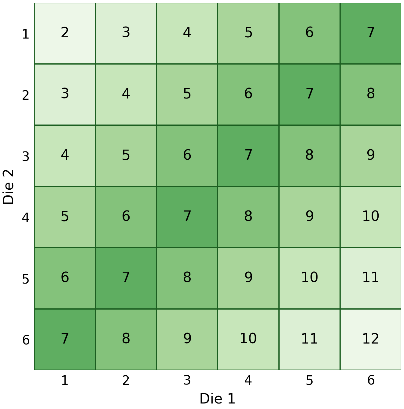
The number of outcomes producing each sum is

\(x\)	Number of outcomes	\(p(x)=P(X=x)\)	\(F(x)=P(X\leq x)\)
2	1	\(1/36\)	\(1/36\)
3	2	\(2/36\)	\(3/36\)
4	3	\(3/36\)	\(6/36\)
5	4	\(4/36\)	\(10/36\)
6	5	\(5/36\)	\(15/36\)
7	6	\(6/36\)	\(21/36\)
8	5	\(5/36\)	\(26/36\)
9	4	\(4/36\)	\(30/36\)
10	3	\(3/36\)	\(33/36\)
11	2	\(2/36\)	\(35/36\)
12	1	\(1/36\)	\(36/36=1\)

This single table contains both the PMF and the CDF. The difference is how the probability is interpreted.

2.2.4 Probability Mass Function

The probability mass function, or PMF, gives the probability at one specific value.

Note

Probability Mass Function

\[p(x)=P(X=x).\]

For the two-dice example,

\[p(7)=P(X=7)=\frac{6}{36}=\frac16.\]

The value 7 has the largest probability because six ordered outcomes produce that sum.

The PMF is shown graphically below.

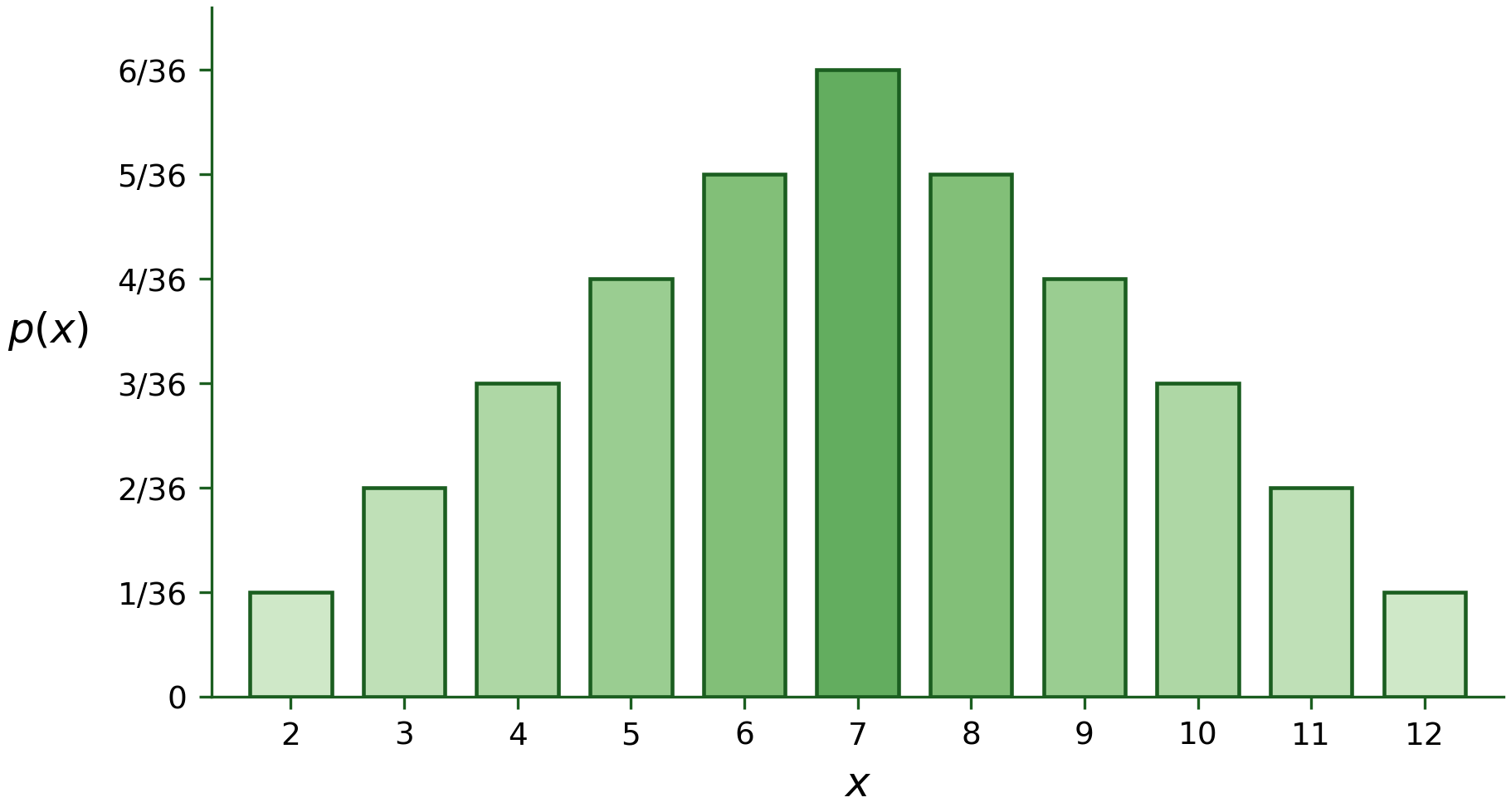
The graph emphasizes two properties of a discrete probability distribution:

• probability is attached to separate possible values of \(X\);

• the possible values do not need to be equally likely.

For example,

\[P(X=2)=\frac{1}{36}, \qquad P(X=7)=\frac{6}{36}.\]

Although both 2 and 7 are possible values, they have different probabilities.

2.2.5 Conditions for a Valid PMF

A PMF must satisfy two conditions.

First,

\[p(x)\geq0\]

for every possible value \(x\).

Second,

\[\sum_x p(x)=1.\]

For the two-dice example,

\[\frac{1+2+3+4+5+6+5+4+3+2+1}{36} = \frac{36}{36} = 1.\]

Therefore, the PMF is valid.

2.2.6 Cumulative Distribution Function

The PMF gives probability at one value. The cumulative distribution function, or CDF, gives probability up to and including a value.

Note

Cumulative Distribution Function

\[F(x)=P(X\leq x).\]

For a discrete random variable, the CDF is obtained by adding PMF probabilities from the smallest possible value up to \(x\).

For example,

\[F(4) = P(X\leq4) = \frac{1+2+3}{36} = \frac{6}{36} = \frac16.\]

Similarly,

\[F(7) = P(X\leq7) = \frac{1+2+3+4+5+6}{36} = \frac{21}{36} = \frac{7}{12}.\]

The CDF therefore accumulates probability as \(x\) moves from left to right.

2.2.7 Why a Discrete CDF Is a Step Function

The CDF is defined for every real value of \(x\), not only for values in the support of \(X\).

For example, the sum of two dice cannot be 6.5. Therefore,

\[F(6.5)=P(X\leq6.5)=P(X\leq6)=F(6).\]

No new probability is added between 6 and 7. The CDF remains constant until the next possible value is reached.

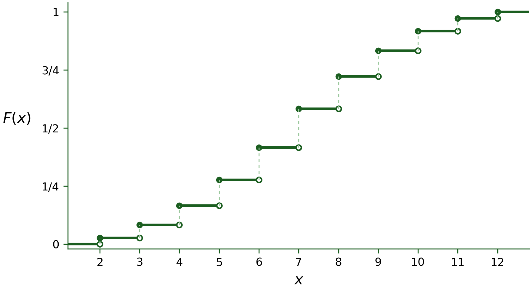
Thus, a discrete CDF is a step function.

At each possible value, the size of the jump equals the PMF probability at that value. For example, the jump at \(x=7\) is

\[p(7)=\frac{6}{36}.\]

This gives the direct connection

\[\text{PMF value} \quad\longleftrightarrow\quad \text{CDF jump size}.\]

2.2.8 Finding Probabilities from the PMF

For probabilities involving several possible values, add the corresponding PMF values.

For example,

\[P(5<X\leq8) = P(X=6)+P(X=7)+P(X=8).\]

Therefore,

\[P(5<X\leq8) = \frac{5+6+5}{36} = \frac{16}{36} = \frac49.\]

2.2.9 Finding Probabilities from the CDF

The same probability can be obtained using cumulative probabilities.

A useful relationship is

\[P(a<X\leq b)=F(b)-F(a).\]

Therefore,

\[P(5<X\leq8) = F(8)-F(5) = \frac{26}{36}-\frac{10}{36} = \frac{16}{36} = \frac49.\]

The CDF is especially convenient for probabilities involving \(\leq\), \(>\), or intervals.

For example,

\[P(X>8) = 1-F(8) = 1-\frac{26}{36} = \frac{10}{36} = \frac{5}{18}.\]

2.2.10 Recovering the PMF from the CDF

For an integer-valued discrete random variable, the probability at a value is the increase in the CDF at that value.

For the two-dice example,

\[p(7) = F(7)-F(6) = \frac{21}{36}-\frac{15}{36} = \frac{6}{36}.\]

Thus, the PMF and CDF contain the same probability information but organize it differently.

2.2.11 PMF Versus CDF

The two functions answer different questions.

Function	Meaning	Example
PMF \(p(x)\)	Probability at one value	\(p(7)=P(X=7)\)
CDF \(F(x)\)	Probability up to and including a value	\(F(7)=P(X\leq7)\)

The PMF appears as separate probability masses or bars.

The discrete CDF appears as a nondecreasing step function.

2.2.12 A Simple Method

For a discrete probability distribution:

1. Define the random variable \(X\).

2. List its possible values.

3. Determine which sample points produce each value.

4. Add their probabilities to obtain \(p(x)\).

5. Check that \(p(x)\geq0\) and \(\sum_x p(x)=1\).

6. Accumulate the PMF from left to right to obtain \(F(x)\).

7. Use the PMF or CDF according to the probability being requested.

2.2.13 Common Mistakes

Do not confuse the value \(X=7\) with the probability \(P(X=7)\).

Do not assume that all possible values are equally likely.

Do not confuse

\[p(x)=P(X=x)\]

with

\[F(x)=P(X\leq x).\]

The PMF gives probability at one value; the CDF gives accumulated probability.

Remember that the CDF is defined for all real values of \(x\), even between possible values of the discrete random variable.

2.2.14 Summary

A discrete probability distribution assigns probabilities to the possible values of a discrete random variable.

The PMF is

\[p(x)=P(X=x),\]

with

\[p(x)\geq0 \qquad\text{and}\qquad \sum_x p(x)=1.\]

The CDF is

\[F(x)=P(X\leq x).\]

For a discrete random variable, the CDF is obtained by accumulating PMF probabilities and therefore appears as a step function.

The size of each CDF jump equals the corresponding PMF probability.